Introduction
We have covered various feature engineering strategies for dealing with structured data in the first two parts of this series. Check out Part-I: Continuous, numeric data and Part-II: Discrete, categorical data for a refresher. In this article, we will look at how to work with text data, which is definitely one of the most abundant sources of unstructured data. Text data usually consists of documents which can represent words, sentences or even paragraphs of free flowing text. The inherent unstructured (no neatly formatted data columns!) and noisy nature of textual data makes it harder for machine learning methods to directly work on raw text data. Hence, in this article, we will follow a hands-on approach to explore some of the most popular and effective strategies for extracting meaningful features from text data. These features can then be used in building machine learning or deep learning models easily.
Motivation
Feature Engineering is often known as the secret sauce to creating superior and better performing machine learning models. Just one excellent feature could be your ticket to winning a Kaggle challenge! The importance of feature engineering is even more important for unstructured, textual data because we need to convert free flowing text into some numeric representations which can then be understood by machine learning algorithms. Even with the advent of automated feature engineering capabilities, you would still need to understand the core concepts behind different feature engineering strategies before applying them as black box models. Always remember, “If you are given a box of tools to repair a house, you should know when to use a power drill and when to use a hammer!”.
Understanding Text Data
I’m sure all of you must be having a fair idea of what textual data comprises of in this scenario. Do remember you can always have text data in the form of structured data attributes, but usually those fall under the umbrella of structured, categorical data.

In this scenario, we are talking about free flowing text in the form of words, phrases, sentences and entire documents. Essentially, we do have some syntactic structure like words make phrases, phrases make sentences which in turn make paragraphs. However, there is no inherent structure to text documents because you can have a wide variety of words which can vary across documents and each sentence will also be of variable length as compared to a fixed number of data dimensions in structured datasets. This article itself is a perfect example of text data!
Feature Engineering Strategies
Let’s look at some popular and effective strategies for handling text data and extracting meaningful features from the same which can be used in downstream machine learning systems. Do note that you can access all the code used in this article in my GitHub repository also for future reference. We’ll start by loading up some basic dependencies and settings.
import pandas as pd
import numpy as np
import re
import nltk
import matplotlib.pyplot as plt
pd.options.display.max_colwidth = 200
%matplotlib inline
Let’s now take a sample corpus of documents on which we will run most of our analyses in this article. A corpus is typically a collection of text documents usually belonging to one or more subjects.
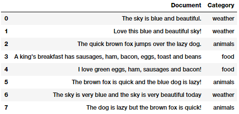
Our sample text corpus
You can see that we have taken a few sample text documents belonging to different categories for our toy corpus. Before we talk about feature engineering, as always, we need to do some data pre-processing or wrangling to remove unnecessary characters, symbols and tokens.

Text pre-processing
There can be multiple ways of cleaning and pre-processing textual data. In the following points, we highlight some of the most important ones which are used heavily in Natural Language Processing (NLP) pipelines.
- Removing tags: Our text often contains unnecessary content like HTML tags, which do not add much value when analyzing text. The BeautifulSoup library does an excellent job in providing necessary functions for this.
- Removing accented characters: In any text corpus, especially if you are dealing with the English language, often you might be dealing with accented characters\letters. Hence we need to make sure that these characters are converted and standardized into ASCII characters. A simple example would be converting é to e.
- Expanding contractions: In the English language, contractions are basically shortened versions of words or syllables. These shortened versions of existing words or phrases are created by removing specific letters and sounds. Examples would be, do not to don’t and I would to I’d. Converting each contraction to its expanded, original form often helps with text standardization.
- Removing special characters: Special characters and symbols which are usually non alphanumeric characters often add to the extra noise in unstructured text. More than often, simple regular expressions (regexes) can be used to achieve this.
- Stemming and lemmatization: Word stems are usually the base form of possible words that can be created by attaching affixes like prefixes and suffixes to the stem to create new words. This is known as inflection. The reverse process of obtaining the base form of a word is known as stemming. A simple example are the words WATCHES, WATCHING, and WATCHED. They have the word root stem WATCH as the base form. Lemmatization is very similar to stemming, where we remove word affixes to get to the base form of a word. However the base form in this case is known as the root word but not the root stem. The difference being that the root word is always a lexicographically correct word (present in the dictionary) but the root stem may not be so.
- Removing stopwords: Words which have little or no significance especially when constructing meaningful features from text are known as stopwords or stop words. These are usually words that end up having the maximum frequency if you do a simple term or word frequency in a corpus. Words like a, an, the, and so on are considered to be stopwords. There is no universal stopword list but we use a standard English language stopwords list from
nltk. You can also add your own domain specific stopwords as needed.

Besides this you can also do other standard operations like tokenization, removing extra whitespaces, text lower casing and more advanced operations like spelling corrections, grammatical error corrections, removing repeated characters and so on. If you are interested, you can check out a sample notebook on text pre-processing from one of my recent books.
Since the focus of this article is on feature engineering, we will build a simple text pre-processor which focuses on removing special characters, extra whitespaces, digits, stopwords and lower casing the text corpus.
Once we have our basic pre-processing pipeline ready, let’s apply the same to our sample corpus.
norm_corpus = normalize_corpus(corpus)
norm_corpus
Output
------
array(['sky blue beautiful', 'love blue beautiful sky',
       'quick brown fox jumps lazy dog',
       'kings breakfast sausages ham bacon eggs toast beans',
       'love green eggs ham sausages bacon',
       'brown fox quick blue dog lazy',
       'sky blue sky beautiful today',
       'dog lazy brown fox quick'],
      dtype='<U51')
The above output should give you a clear view of how each of our sample documents look like after pre-processing. Let’s engineer some features now!
Bag of Words Model
This is perhaps the most simple vector space representational model for unstructured text. A vector space model is simply a mathematical model to represent unstructured text (or any other data) as numeric vectors, such that each dimension of the vector is a specific feature\attribute. The bag of words model represents each text document as a numeric vector where each dimension is a specific word from the corpus and the value could be its frequency in the document, occurrence (denoted by 1 or 0) or even weighted values. The model’s name is such because each document is represented literally as a ‘bag’ of its own words, disregarding word orders, sequences and grammar.
Output
------
array([[0, 0, 1, 1, 0, 0, 0, 0, 0, 0, 0, 0, 0, 0, 0, 0, 0, 1, 0, 0],
       [0, 0, 1, 1, 0, 0, 0, 0, 0, 0, 0, 0, 0, 0, 1, 0, 0, 1, 0, 0],
       [0, 0, 0, 0, 0, 1, 1, 0, 1, 0, 0, 1, 0, 1, 0, 1, 0, 0, 0, 0],
       [1, 1, 0, 0, 1, 0, 0, 1, 0, 0, 1, 0, 1, 0, 0, 0, 1, 0, 1, 0],
       [1, 0, 0, 0, 0, 0, 0, 1, 0, 1, 1, 0, 0, 0, 1, 0, 1, 0, 0, 0],
       [0, 0, 0, 1, 0, 1, 1, 0, 1, 0, 0, 0, 0, 1, 0, 1, 0, 0, 0, 0],
       [0, 0, 1, 1, 0, 0, 0, 0, 0, 0, 0, 0, 0, 0, 0, 0, 0, 2, 0, 1],
       [0, 0, 0, 0, 0, 1, 1, 0, 1, 0, 0, 0, 0, 1, 0, 1, 0, 0, 0, 0]
      ], dtype=int64)
Thus you can see that our documents have been converted into numeric vectors such that each document is represented by one vector (row) in the above feature matrix. The following code will help represent this in a more easy to understand format.
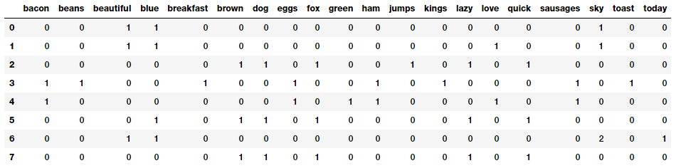
Our Bag of Words model based document feature vectors
This should make things more clearer! You can clearly see that each column or dimension in the feature vectors represents a word from the corpus and each row represents one of our documents. The value in any cell, represents the number of times that word (represented by column) occurs in the specific document (represented by row). Hence if a corpus of documents consists of Nunique words across all the documents, we would have an N-dimensionalvector for each of the documents.
Bag of N-Grams Model
A word is just a single token, often known as a unigram or 1-gram. We already know that the Bag of Words model doesn’t consider order of words. But what if we also wanted to take into account phrases or collection of words which occur in a sequence? N-grams help us achieve that. An N-gram is basically a collection of word tokens from a text document such that these tokens are contiguous and occur in a sequence. Bi-grams indicate n-grams of order 2 (two words), Tri-grams indicate n-grams of order 3 (three words), and so on. The Bag of N-Grams model is hence just an extension of the Bag of Words model so we can also leverage N-gram based features. The following example depicts bi-gram based features in each document feature vector.
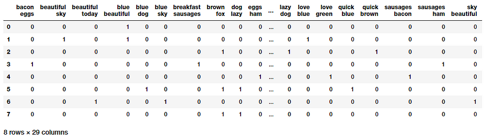
Bi-gram based feature vectors using the Bag of N-Grams Model
This gives us feature vectors for our documents, where each feature consists of a bi-gram representing a sequence of two words and values represent how many times the bi-gram was present for our documents.
TF-IDF Model
There are some potential problems which might arise with the Bag of Words model when it is used on large corpora. Since the feature vectors are based on absolute term frequencies, there might be some terms which occur frequently across all documents and these may tend to overshadow other terms in the feature set. The TF-IDF model tries to combat this issue by using a scaling or normalizing factor in its computation. TF-IDF stands for Term Frequency-Inverse Document Frequency, which uses a combination of two metrics in
its computation, namely: term frequency (tf) and inverse document frequency (idf). This technique was developed for ranking results for queries in search engines and now it is an indispensable model in the world of information retrieval and NLP.
Mathematically, we can define TF-IDF as tfidf = tf x idf, which can be expanded further to be represented as follows.
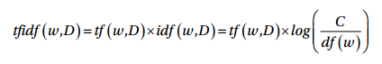
Here, tfidf(w, D) is the TF-IDF score for word w in document D. The term tf(w, D) represents the term frequency of the word w in document D, which can be obtained from the Bag of Words model. The term idf(w, D) is the inverse document frequency for the term w, which can be computed as the log transform of the total number of documents in the corpus C divided by the document frequency of the word w, which is basically the frequency of documents in the corpus where the word w occurs. There are multiple variants of this model but they all end up giving quite similar results. Let’s apply this on our corpus now!
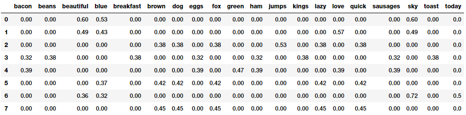
Our TF-IDF model based document feature vectors
The TF-IDF based feature vectors for each of our text documents show scaled and normalized values as compared to the raw Bag of Words model values. Interested readers who might want to dive into further details of how the internals of this model work can refer to page 181 of Text Analytics with Python (Springer\Apress; Dipanjan Sarkar, 2016).
Document Similarity
Document similarity is the process of using a distance or similarity based metric that can be used to identify how similar a text document is with any other document(s) based on features extracted from the documents like bag of words or tf-idf.

Are we similar?
Thus you can see that we can build on top of the tf-idf based features we engineered in the previous section and use them to generate new features which can be useful in domains like search engines, document clustering and information retrieval by leveraging these similarity based features.
Pairwise document similarity in a corpus involves computing document similarity for each pair of documents in a corpus. Thus if you have C documents in a corpus, you would end up with a C x C matrix such that each row and column represents the similarity score for a pair of documents, which represent the indices at the row and column, respectively. There are several similarity and distance metrics that are used to compute document similarity. These include cosine distance/similarity, euclidean distance, manhattan distance, BM25 similarity, jaccard distance and so on. In our analysis, we will be using perhaps the most popular and widely used similarity metric,
cosine similarity and compare pairwise document similarity based on their TF-IDF feature vectors.
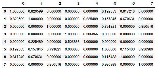
Pairwise document similarity matrix (cosine similarity)
Cosine similarity basically gives us a metric representing the cosine of the angle between the feature vector representations of two text documents. Lower the angle between the documents, the closer and more similar they are as depicted in the following figure.
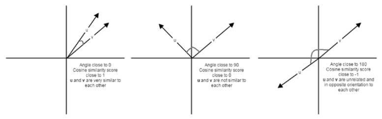
Cosine similarity depictions for text document feature vectors
Looking closely at the similarity matrix clearly tells us that documents (0, 1 and 6), (2, 5 and 7) are very similar to one another and documents 3 and 4 are slightly similar to each other but the magnitude is not very strong, however still stronger than the other documents. This must indicate these similar documents have some similar features. This is a perfect example of grouping or clustering that can be solved by unsupervised learning especially when you are dealing with huge corpora of millions of text documents.
Document Clustering with Similarity Features
Clustering leverages unsupervised learning to group data points (documents in this scenario) into groups or clusters. We will be leveraging an unsupervised hierarchical clustering algorithm here to try and group similar documents from our toy corpus together by leveraging the document similarity features we generated earlier. There are two types of hierarchical clustering algorithms namely, agglomerative and divisive methods. We will be using a agglomerative clustering algorithm, which is hierarchical clustering using a bottom up approach i.e. each observation or document starts in its own cluster and clusters are successively merged together using a distance metric which measures distances between data points and a linkage merge criterion. A sample depiction is shown in the following figure.
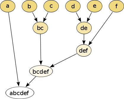
Agglomerative Hierarchical Clustering
The selection of the linkage criterion governs the merge strategy. Some examples of linkage criteria are Ward, Complete linkage, Average linkage and so on. This criterion is very useful for choosing the pair of clusters (individual documents at the lowest step and clusters in higher steps) to merge at each step is based on the optimal value of an objective function. We choose the Ward’s minimum variance method as our linkage criterion to minimize total within-cluster variance. Hence, at each step, we find the pair of clusters that leads to minimum increase in total within-cluster variance after merging. Since we already have our similarity features, let’s build out the linkage matrix on our sample documents.
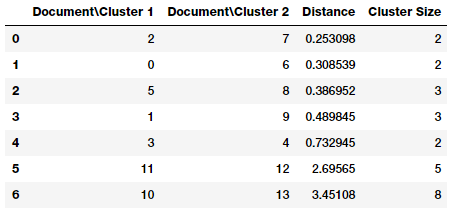
Linkage Matrix for our Corpus
If you closely look at the linkage matrix, you can see that each step (row) of the linkage matrix tells us which data points (or clusters) were merged together. If you have n data points, the linkage matrix, Z will be having a shape of (n — 1) x 4 where Z[i] will tell us which clusters were merged at step i. Each row has four elements, the first two elements are either data point identifiers or cluster labels (in the later parts of the matrix once
multiple data points are merged), the third element is the cluster distance between the first two elements (either data points or clusters), and the last element is the total number of elements\data points in the cluster once the merge is complete. We recommend you refer to the scipy documentation, which explains this in detail.
Let’s now visualize this matrix as a dendrogram to understand the elements better!
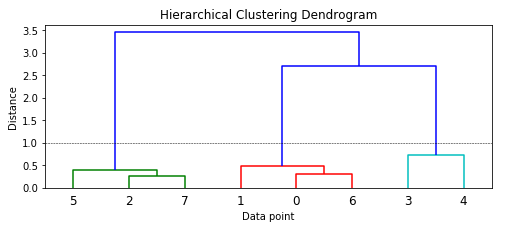
Dendrogram visualizing our hierarchical clustering process
We can see how each data point starts as an individual cluster and slowly starts getting merged with other data points to form clusters. On a high level from the colors and the dendrogram, you can see that the model has correctly identified three major clusters if you consider a distance metric of around 1.0or above (denoted by the dotted line). Leveraging this distance, we get our cluster labels.
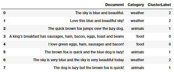
Clustering our documents into groups with hierarchical clustering
Thus you can clearly see our algorithm has correctly identified the three distinct categories in our documents based on the cluster labels assigned to them. This should give you a good idea of how our TF-IDF features were leveraged to build our similarity features which in turn helped in clustering our documents. You can actually use this pipeline in the future for clustering your own documents!
Topic Models
We can also use some summarization techniques to extract topic or concept based features from text documents. The idea of topic models revolves around the process of extracting key themes or concepts from a corpus of documents which are represented as topics. Each topic can be represented as a bag or collection of words/terms from the document corpus. Together, these terms signify a specific topic, theme or a concept and each topic can be easily distinguished from other topics by virtue of the semantic meaning conveyed by these terms. However often you do end up with overlapping topics based on the data. These concepts can range from simple facts and statements to opinions and outlook. Topic models are extremely useful in summarizing large corpus of text documents to extract and depict key concepts. They are also useful in extracting features from text data that capture latent patterns in the data.
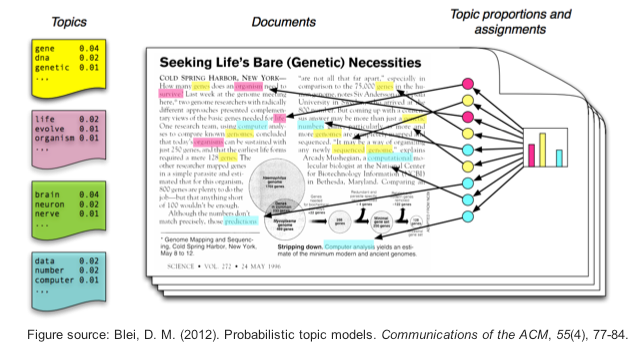
An example of topic models
There are various techniques for topic modeling and most of them involve some form of matrix decomposition. Some techniques like Latent Semantic Indexing (LSI) use matrix decomposition operations, more specifically Singular Valued Decomposition. We will be using another technique is Latent Dirichlet Allocation (LDA), which uses a generative probabilistic model where each document consists of a combination of several topics and each term or word can be assigned to a specific topic. This is similar to pLSI based model (probabilistic LSI). Each latent topic contains a Dirichlet prior over them in the case of LDA.
The math behind in this technique is pretty involved, so I will try to summarize it without boring you with a lot of details. I recommend readers to go through this excellent talk by Christine Doig.
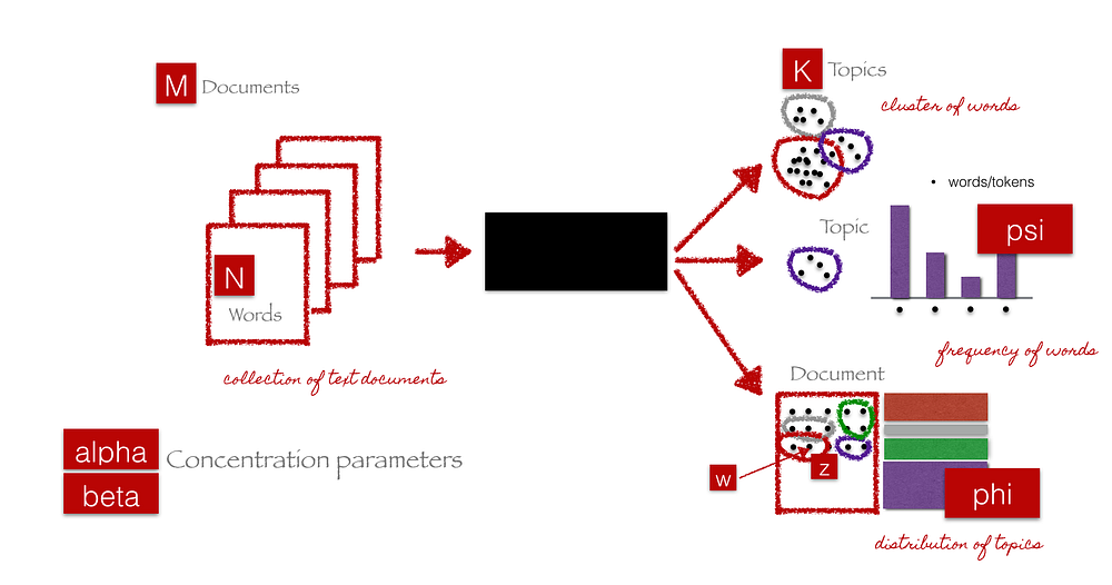
End-to-end LDA framework (courtesy of C. Doig, Introduction to Topic
Modeling in Python)
The black box in the above figure represents the core algorithm that makes use of the previously mentioned parameters to extract K topics from Mdocuments. The following steps give a simplistic explanation of what happens in the algorithm behind the scenes.
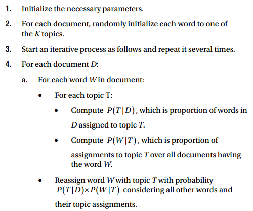
Once this runs for several iterations, we should have topic mixtures for each document and then generate the constituents of each topic from the terms that point to that topic. Frameworks like gensim or scikit-learn enable us to leverage the LDA model for generating topics.
For the purpose of feature engineering which is the intent of this article, you need to remember that when LDA is applied on a document-term matrix (TF-IDF or Bag of Words feature matrix), it gets decomposed into two main components.
- A document-topic matrix, which would be the feature matrix we
are looking for. - A topic-term matrix, which helps us in looking at potential topics in the corpus.
Let’s leverage scikit-learn to get the document-topic matrix as follows.
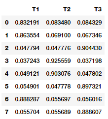
Document-Topic Matrix from our LDA Model
You can clearly see which documents contribute the most to which of the three topics in the above output. You can view the topics and their main constituents as follows.
Topic 1
-------
[('sky', 4.3324395825632624), ('blue', 3.3737531748317711), ('beautiful', 3.3323652405224857), ('today', 1.3325579841038182), ('love', 1.3304224288080069)]
Topic 2
-------
[('bacon', 2.3326959484799978), ('eggs', 2.3326959484799978), ('ham', 2.3326959484799978), ('sausages', 2.3326959484799978), ('love', 1.335454457601996), ('beans', 1.3327735253784641), ('breakfast', 1.3327735253784641), ('kings', 1.3327735253784641), ('toast', 1.3327735253784641), ('green', 1.3325433207547732)]
Topic 3
-------
[('brown', 3.3323474595768783), ('dog', 3.3323474595768783), ('fox', 3.3323474595768783), ('lazy', 3.3323474595768783), ('quick', 3.3323474595768783), ('jumps', 1.3324193736202712), ('blue', 1.2919635624485213)]
Thus you can clearly see the three topics are quite distinguishable from each other based on their constituent terms, first one talking about weather, second one about food and the last one about animals. Choosing the number of topics for topic modeling is an entire topic on its own (pun not intended!) and is an art as well as a science. There are various methods and heuristics to get the optimal number of topics but due to the detailed nature of these techniques, we don’t discuss them here.
Document Clustering with Topic Model Features
We used our Bag of Words model based features to build out topic model based features using LDA. We can now actually leverage the document term matrix we obtained and use an unsupervised clustering algorithm to try and group our documents similar to what we did earlier with our similarity features.
We will use a very popular partition based clustering method this time, K-means clustering to cluster or group these documents based on their topic model feature representations. In K-means clustering, we have an input parameter k, which specifies the number of clusters it will output using the document features. This clustering method is a centroid based clustering method, where it tries to cluster these documents into clusters of equal variance. It tries to create these clusters by minimizing the within-cluster sum of squares measure, also known as inertia. There are multiple ways to select the optimal value of k like using the Sum of Squared Errors metric, Silhouette Coefficients and the Elbow method.
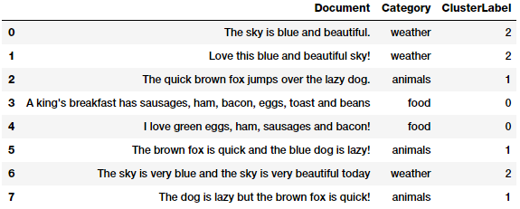
Clustering our documents into groups with K-means clustering
We can see from the above output that our documents were correctly assigned to the right clusters!
Future Scope for Advanced Strategies
What we didn’t cover in this article are several advanced strategies around feature engineering for text data which have recently come into prominence. This includes leveraging deep learning based models to obtain word embeddings. We will take a deep dive into such models in the next part of this series and cover popular word embedding models like Word2Vec and GloVewith detailed hands-on examples so stay tuned!
Conclusion
These examples should give you a good idea about popular strategies for feature engineering on text data. Do remember that these are traditional strategies based on concepts from mathematics, information retrieval and natural language processing. Hence these tried and tested methods over time have proven to be successful in a wide variety of datasets and problems. Next up will be detailed strategies on leveraging deep learning models for feature engineering on text data!
To read about feature engineering strategies for continuous numeric data, check out Part 1 of this series!
To read about feature engineering strategies for discrete categoricial data, check out Part 2 of this series!
All the code and datasets used in this article can be accessed from my GitHub
The code is also available as a Jupyter notebook