ssim的计算里面有高斯模糊

为了快速计算，先对每个小块进行计算，然后计算所有块的平均值。

可以参考源代码实现，而且代码实现有近似的在里面！matlab中中图像PSNR和SSIM的计算

“在实际应用中，可以利用滑动窗将图像分块，令分块总数为N，考虑到窗口形状对分块的影响，采用高斯加权计算每一窗口的均值、方差以及协方差，然后计算对应块的结构相似度SSIM，最后将平均值作为两图像的结构相似性度量，即平均结构相似性MSSIM”

function [mssim, ssim_map] = ssim(img1, img2, K, window, L)

% ========================================================================
% SSIM Index with automatic downsampling, Version 1.0
% Copyright(c) 2009 Zhou Wang
% All Rights Reserved.
%
% ----------------------------------------------------------------------
% Permission to use, copy, or modify this software and its documentation
% for educational and research purposes only and without fee is hereby
% granted, provided that this copyright notice and the original authors'
% names appear on all copies and supporting documentation. This program
% shall not be used, rewritten, or adapted as the basis of a commercial
% software or hardware product without first obtaining permission of the
% authors. The authors make no representations about the suitability of
% this software for any purpose. It is provided "as is" without express
% or implied warranty.
%----------------------------------------------------------------------
%
% This is an implementation of the algorithm for calculating the
% Structural SIMilarity (SSIM) index between two images
%
% Please refer to the following paper and the website with suggested usage
%
% Z. Wang, A. C. Bovik, H. R. Sheikh, and E. P. Simoncelli, "Image
% quality assessment: From error visibility to structural similarity,"
% IEEE Transactios on Image Processing, vol. 13, no. 4, pp. 600-612,
% Apr. 2004.
%
% http://www.ece.uwaterloo.ca/~z70wang/research/ssim/
%
% Note: This program is different from ssim_index.m, where no automatic
% downsampling is performed. (downsampling was done in the above paper
% and was described as suggested usage in the above website.)
%
% Kindly report any suggestions or corrections to [email protected]
%
%----------------------------------------------------------------------
%
%Input : (1) img1: the first image being compared
% (2) img2: the second image being compared
% (3) K: constants in the SSIM index formula (see the above
% reference). defualt value: K = [0.01 0.03]
% (4) window: local window for statistics (see the above
% reference). default widnow is Gaussian given by
% window = fspecial('gaussian', 11, 1.5);
% (5) L: dynamic range of the images. default: L = 255
%
%Output: (1) mssim: the mean SSIM index value between 2 images.
% If one of the images being compared is regarded as
% perfect quality, then mssim can be considered as the
% quality measure of the other image.
% If img1 = img2, then mssim = 1.
% (2) ssim_map: the SSIM index map of the test image. The map
% has a smaller size than the input images. The actual size
% depends on the window size and the downsampling factor.
%
%Basic Usage:
% Given 2 test images img1 and img2, whose dynamic range is 0-255
%
% [mssim, ssim_map] = ssim(img1, img2);
%
%Advanced Usage:
% User defined parameters. For example
%
% K = [0.05 0.05];
% window = ones(8);
% L = 100;
% [mssim, ssim_map] = ssim(img1, img2, K, window, L);
%
%Visualize the results:
%
% mssim %Gives the mssim value
% imshow(max(0, ssim_map).^4) %Shows the SSIM index map
%========================================================================

if (nargin < 2 || nargin > 5)
mssim = -Inf;
ssim_map = -Inf;
return;
end

if (size(img1) ~= size(img2))
mssim = -Inf;
ssim_map = -Inf;
return;
end

[M,N] = size(img1);

if (nargin == 2)
if ((M < 11) || (N < 11)) %图像尺寸大小太小没有意义
mssim = -Inf;
ssim_map = -Inf;
return
end
window = fspecial('gaussian', 11, 1.5); %标准偏差为1.5 ， 11*11的高斯低通滤波器
K(1) = 0.01; % default settings
K(2) = 0.03; %
L = 255; %
end

if (nargin == 3)
if ((M < 11) || (N < 11))
mssim = -Inf;
ssim_map = -Inf;
return
end
window = fspecial('gaussian', 11, 1.5);
L = 255;
if (length(K) == 2)
if (K(1) < 0 || K(2) < 0)
mssim = -Inf;
ssim_map = -Inf;
return;
end
else
mssim = -Inf;
ssim_map = -Inf;
return;
end
end

if (nargin == 4)
[H,W] = size(window);
if ((H*W) < 4 || (H > M) || (W > N))
mssim = -Inf;
ssim_map = -Inf;
return
end
L = 255;
if (length(K) == 2)
if (K(1) < 0 || K(2) < 0)
mssim = -Inf;
ssim_map = -Inf;
return;
end
else
mssim = -Inf;
ssim_map = -Inf;
return;
end
end

if (nargin == 5)
[H,W] = size(window);
if ((H*W) < 4 || (H > M) || (W > N))
mssim = -Inf;
ssim_map = -Inf;
return
end
if (length(K) == 2)
if (K(1) < 0 || K(2) < 0)
mssim = -Inf;
ssim_map = -Inf;
return;
end
else
mssim = -Inf;
ssim_map = -Inf;
return;
end
end

img1 = double(img1);
img2 = double(img2);

% automatic downsampling
f = max(1,round(min(M,N)/256));
%downsampling by f
%use a simple low-pass filter
if(f>1)
lpf = ones(f,f);
lpf = lpf/sum(lpf(:));
img1 = imfilter(img1,lpf,'symmetric','same');
img2 = imfilter(img2,lpf,'symmetric','same');

img1 = img1(1:f:end,1:f:end);
img2 = img2(1:f:end,1:f:end);
end

C1 = (K(1)*L)^2;
C2 = (K(2)*L)^2;
window = window/sum(sum(window));

mu1 = filter2(window, img1, 'valid');
mu2 = filter2(window, img2, 'valid');
mu1_sq = mu1.*mu1;
mu2_sq = mu2.*mu2;
mu1_mu2 = mu1.*mu2;
sigma1_sq = filter2(window, img1.*img1, 'valid') - mu1_sq;
sigma2_sq = filter2(window, img2.*img2, 'valid') - mu2_sq;
sigma12 = filter2(window, img1.*img2, 'valid') - mu1_mu2;

if (C1 > 0 && C2 > 0)
ssim_map = ((2*mu1_mu2 + C1).*(2*sigma12 + C2))./((mu1_sq + mu2_sq + C1).*(sigma1_sq + sigma2_sq + C2));
else
numerator1 = 2*mu1_mu2 + C1;
numerator2 = 2*sigma12 + C2;
denominator1 = mu1_sq + mu2_sq + C1;
denominator2 = sigma1_sq + sigma2_sq + C2;
ssim_map = ones(size(mu1));
index = (denominator1.*denominator2 > 0);
ssim_map(index) = (numerator1(index).*numerator2(index))./(denominator1(index).*denominator2(index));
index = (denominator1 ~= 0) & (denominator2 == 0);
ssim_map(index) = numerator1(index)./denominator1(index);
end

mssim = mean2(ssim_map);

return

PSNR , 峰值信噪比

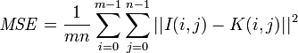
通常用来评价一幅图像压缩后和原图像相比质量的好坏，当然，压缩后图像一定会比原图像质量差的，所以就用这样一个评价指标来规定标准了。PSNR越高，压缩后失真越小。这里主要定义了两个值，一个是均方差MSE，另一个是峰值信噪比PSNR，公式如下：

PSNR越高，图像和原图越接近。当然，这都是客观指标，实际评价还有主观指标，不过主观的东西就比较模糊了，每个人感觉都会不同的。最常用的全参考视频质量评价方法有以下2种：

PSNR（峰值信噪比）：用得最多，但是其值不能很好地反映人眼主观感受。一般取值范围：20-40.值越大，视频质量越好。

SSIM（结构相似性）：计算稍复杂，其值可以较好地反映人眼主观感受。一般取值范围：0-1.值越大，视频质量越好。

PSNR，SSIM计算有如下工具可选：

MSU Video Quality Measurement Tool：商业软件，图形化界面，易上手，使用有限制。

Evalvid中的psnr.exe：开源软件，命令行界面，使用无限制。推荐，适合批处理。

偶然发现了一个很好的网站。里面包含了大量主观评价算法的数据，导入到Matlab中就可以使用。http://sse.tongji.edu.cn/linzhang/IQA/IQA.htm

注：MOS（Mean Opnion Score，平均意见分）是主观评价实验之后，得到的主观分数，取值0-100，值越大，代表主观感受越好。以下实验数据来自Live数据库：http://live.ece.utexas.edu/research/Quality/

SSIM参数

一种衡量两幅图像相似度的新指标，其值越大越好，最大为1，经常用到图像处理中，特别在图像去噪处理中在图像相似度评价上全面超越SNR（signal to noise ratio）和PSNR（peak signal to noise ratio）。

结构相似性理论认为，自然图像信号是高度结构化的，即像素间有很强的相关性，特别是空域中最接近的像素，这种相关性蕴含着视觉场景中物体结构的重要信息；

HVS的主要功能是从视野中提取结构信息，可以用对结构信息的度量作为图像感知质量的近似。结构相似性理论是一种不同于以往模拟HVS低阶的组成结构的全新思想，与基于HVS特性的方法相比，最大的区别是自顶向下与自底向上的区别。这一新思想的关键是从对感知误差度量到对感知结构失真度量的转变。它没有试图通过累加与心理物理学简单认知模式有关的误差来估计图像质量，而是直接估计两个复杂结构信号的结构改变，从而在某种程度上绕开了自然图像内容复杂性及多通道去相关的问题。作为结构相似性理论的实现，结构相似度指数从图像组成的角度将结构信息定义为独立于亮度、对比度的，反映场景中物体结构的属性，并将失真建模为亮度、对比度和结构三个不同因素的组合。用均值作为亮度的估计，标准差作为对比度的估计，协方差作为结构相似程度的度量。

结构相似性指标(英文： structural similarity index， SSIM index)是一种用以衡量两张数位影像相似程度的指标。当两张影像其中一张为无失真影像，另一张为失真后的影像，二者的结构相似性可以看成是失真影像的影像品质衡量指标。相较于传统所使用的影像品质衡量指标，像是峰值信噪比(英文： PSNR)，结构相似性在影像品质的衡量上更能符合人眼对影像品质的判断。

实际使用时，简化起见，一般会将参数设为 $\alpha=\beta=\gamma=1$ 及 $C_3=C_2/2$ ，得到：

$\text{SSIM}(\mathbf{x},\mathbf{y})=\frac{(2\mu_x\mu_y+C_1)(2\sigma_{xy}+C_2)}{(\mu_x^2+\mu_y^2+C_1)(\sigma_x^2+\sigma_y^2+C_2)}$

在计算两张影像的结构相似性指标时，会开一个局部性的视窗，一般为 $N$ × $N$ 的小区块，计算出视窗内信号的结构相似性指标，每次以像素为单位移动视窗，直到整张影像每个位置的局部结构相似性指标都计算完毕。将全部的局部结构相似性指标平均起来即为两张影像的结构相似性指标。

在实际应用中，可以利用滑动窗将图像分块，令分块总数为N，考虑到窗口形状对分块的影响，采用高斯加权计算每一窗口的均值、方差以及协方差，然后计算对应块的结构相似度SSIM，最后将平均值作为两图像的结构相似性度量，即平均结构相似性MSSIM:

opencv和matlab都有现成的函数可以使用。

参考：图像质量评价--SSIM

全参考视频质量评价方法（PSNR，SSIM）以及相关数据库

图像质量评价指标

update 2018-07-0716:50:16
均方误差(MSE)和均方根误差(RMSE)和平均绝对误差(MAE)

MSE: Mean Squared Error
均方误差是指参数估计值与参数真值之差平方的期望值;
MSE可以评价数据的变化程度，MSE的值越小，说明预测模型描述实验数据具有更好的精确度。

RMSE
均方误差:均方根误差是均方误差的算术平方根

MAE :Mean Absolute Error
平均绝对误差是绝对误差的平均值
平均绝对误差能更好地反映预测值误差的实际情况.

SD :standard Deviation
标准差:标准差是方差的算术平方根。标准差能反映一个数据集的离散程度。平均数相同的两组组数据，标准差未必相同。

评估图像质量评价算法性能的几个常用的标准

Spearman秩序相关系数（SROCC）本身就不是衡量线性相关的，而是衡量秩序的相关性的。设有两组序列X和Y，其秩序为R(X)和R(Y)，这里R(Xi)=k代表Xi是序列X中的第k大（或第k小），则SROCC(X, Y) = PLCC(R(X), R(Y))，其中PLCC是Pearson线性相关系数。
SROCC被认为是最好的非线性相关指标，这是因为，SROCC只与序列中元素的排序有关。因此即使X或Y被任何单调非线性变换作用（如对数变换、指数变换），都不会对SROCC造成任何影响，因为不会影响元素的排序。维基百科有一张很直观的图片，很好地体现了SROCC与PLCC的区别。

除此之外，还有一个Kendall秩序相关系数（KROCC），它的定义是pairwise的：
KROCC = (同序对数-逆序对数) / 总对数（总对数=n(n - 1)/2）它的性质与SROCC类似，但是比较抖。

对于连续输出的机器学习模型或简单的回归拟合，发Paper的话，一般要放SROCC和PLCC，这两个标准是最重要的，可以很好地衡量模型的非线性相关性和线性相关性。偶尔也会放KROCC和RMSE（方均根误差）。但是SROCC是比PLCC更为根本的指标，因为一个复杂模型总可以用一些附加的非线性变换（对数或者指数，还有某些领域内recommanded复杂的组合= =）来补正，使得PLCC更高一些，而SROCC却不能被这些附加非线性变换来影响。

图像质量评价相关收录

图像质量评价指标

猜你喜欢