利用python实现梯度下降和逻辑回归原理(Python详细源码：预测学生是否被录取)

本案例主要是：建立逻辑回归模型预测一个学生是否被大学录取，没有详细介绍算法推到，

读者可查阅其他博客理解梯度下降算法的实现：https://blog.csdn.net/wangliang0633/article/details/79082901

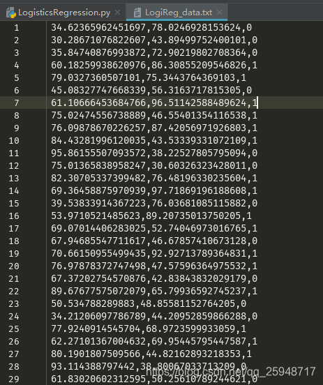
数据格式如下：第三列表示录取状态，0---未录取，1---已录取，前两列是成绩

源码：

#!/usr/bin/env python
# encoding: utf-8
"""
@Company：华中科技大学电气学院聚变与等离子研究所
@version: V1.0
@author: Victor
@contact: [email protected] or [email protected] 2018--2020
@software: PyCharm
@file: LogisticsRegression.py
@time: 2018/11/12 15:10
@Desc：建立逻辑回归模型预测一个学生是否被大学录取
"""
import numpy as np
import pandas as pd
import matplotlib.pyplot as plt

import os
path="E:\PycharmWorks\Files"+os.sep+"LogiReg_data.txt"
pdData = pd.read_csv(path,header=None,names=['Exam1','Exam2','Admitted'])
#pdData.head(3)

##画出录取和未录取的散点分布图
positive = pdData[pdData['Admitted'] == 1]
negative = pdData[pdData['Admitted'] == 0]

#plt.scatter(positive['Exam1'],positive['Exam2'],s=30,c='b',marker='o',label='Admitted')
#plt.scatter(negative['Exam1'],negative['Exam2'],s=30,c='r',marker='x',label='UNAdmitted')

#plt.legend()
#plt.xlabel("Exam1 Score")
#plt.ylabel("Exam2 Score")
#plt.show()

'''目标：建立分类器
   设定阈值：根据阈值判断录取结果
   要完成的模块：
      sigmodi:映射到概率的函数
      model:返回预测结果值
      cost：根据参数计算损失
      gradient：计算每个参数的梯度方向
      descent：进行参数更新
      accuracy：计算精度'''


def sigmoid(z):
    return 1/(1+np.exp(-z))

def model(X,theta):
    return sigmoid(np.dot(X,theta.T))

pdData.insert(0,'Ones',1)
#print(pdData)

orig_data = pdData.as_matrix() ##变为矩阵
##print(orig_data)
cols = orig_data.shape[1]
X = orig_data[:,0:cols-1]
#print(X[:5]) ##前5行
y = orig_data[:,cols-1:cols]
#print(y[:4])
##构建参数矩阵
theta = np.zeros([1,3])
#print(theta)

####损失函数（实现似然函数）,
def cost(X,y,theta):
    left = np.multiply(-y,np.log(model(X,theta)))
    right = np.multiply(1 - y,np.log(1 - model(X,theta)))
    return np.sum(left-right)/(len(X))/n

#print(cost(X,y,theta))

####计算梯度,计算每个参数的梯度
def gradient(X,y,theta):
    grad = np.zeros(theta.shape) ##占位
    error = (model(X,theta)-y)[:,1]
    for j in range(len(theta.ravel())):
        term = np.multiply(error,X[:,j])###X的行表示样本，列表示特征
        grad[0,j] = np.sum(term) / len(X)
    return grad


#print(gradient(X,y,theta))

###比较三种不同的梯度下降方法
STOP_ITER = 0
STOP_COST = 1
STOP_GRAD = 2

def stopCriterion(type,value,threshod):
    if type == STOP_ITER: return value > threshod
    elif type == STOP_COST: return abs(value[-1]-value[-2] < threshod)
    elif type == STOP_GRAD: return np.linalg.norm(value) < threshod


###洗牌,避免数据收集过程中有规律，打乱数据，可以得到更好的模型
import numpy.random
def shuffleData(data):
    np.random.shuffle(data)
    cols = data.shape[1]
    X = data[:,0:cols-1]
    y = data[:,cols-1]
    return X,y

####梯度下降求解
import time
def descent(data,theta,batchSize,stopType,thresh,alpha):
    init_time = time.time()
    i = 0 #迭代次数
    k = 0 #batch
    X,y = shuffleData(data)
    grad = np.zeros(theta.shape)
    costs = [cost(X,y,theta)]

    while True:
        grad = gradient(X[k:k+batchSize],y[k:k+batchSize],theta)
        k += batchSize
        if k >= 100:
           k = 0
           X,y = shuffleData(data)
        theta = theta -alpha*grad ##参数更新
        costs.append(cost(X,y,theta)) ##计算新的损失
        i += 1

        if stopType == STOP_ITER: value = i
        elif stopType == STOP_COST: value = costs
        elif stopType == STOP_GRAD: value = grad
        if stopCriterion(stopType,value,thresh):break

    return theta,i-1,costs,grad,time.time()-init_time


def RunExp(data,theta,batchSize,stopType,thresh,alpha):
    theta,iter,costs,grad,dur = descent(data,theta,batchSize,stopType,thresh,alpha)
    name = "Original" if (data[:,1]>2).sum() > 1 else "Scaled"
    name += "data- learning rate:{}-".format(alpha)

    print("***{}\nTheta:{}-Iter:{}-Last cost:{:03.2f} - Duration:{:03.2f}s".format(name,theta,iter,costs[-1],dur))

    plt.plot(np.arange(len(costs)),costs,'r')
    plt.xlabel("Iterations")
    plt.ylabel("Cost")
    plt.title("Error vs Itetarion")
    plt.show()
    return theta

n=100
RunExp(orig_data,theta,n,STOP_ITER,thresh=12000,alpha=0.00000012)

###计算模型精度


##设定阈值
def predict(X,theta):
    return [1 if x >= 0.5 else  0 for x in model(X,theta)]

scaled_X = orig_data[:,:3]
y = orig_data[:,3]
predicts = predict(scaled_X,theta)

correct = [1 if ((a == 1 and b == 1) or (a == 0 and b == 0)) else 0 for (a,b) in zip(predicts,y)]
accuracy = (correct.count(1) % len(correct))
print("accuracy = {0}%".format(accuracy))

结果显示：

结果预测：

可见准确率不高，还需调整参数，增加样本。