基于决策树模型对 IRIS 数据集分类

基于决策树模型对 IRIS 数据集分类

1 python 实现

加载数据集

IRIS 数据集在 sklearn 模块中已经提供。

# -*- coding: utf-8 -*-

from matplotlib import pyplot as plt
import numpy as np
from sklearn import tree
from sklearn.datasets import load_iris

if __name__ == '__main__':
    print('\n\n\n\n\n\n\n\n\n\n')

    # show data info
    data = load_iris() # 加载 IRIS 数据集
    print('keys: \n', data.keys()) # ['data', 'target', 'target_names', 'DESCR', 'feature_names']
    feature_names = data.get('feature_names')
    print('feature names: \n', data.get('feature_names')) # 查看属性名称
    print('target names: \n', data.get('target_names')) # 查看 label 名称
    x = data.get('data') # 获取样本矩阵
    y = data.get('target') # 获取与样本对应的 label 向量
    print(x.shape, y.shape) # 查看样本数据
    print(data.get('DESCR'))

可视化数据集

# visualize the data
    f = []
    f.append(y==0) # 类别为第一类的样本的逻辑索引
    f.append(y==1) # 类别为第二类的样本的逻辑索引
    f.append(y==2) # 类别为第三类的样本的逻辑索引
    color = ['red','blue','green']
    fig, axes = plt.subplots(4,4) # 绘制四个属性两辆之间的散点图
    for i, ax in enumerate(axes.flat):
        row  = i // 4
        col = i % 4
        if row == col:
            ax.text(.1,.5, feature_names[row])
            ax.set_xticks([])
            ax.set_yticks([])
            continue
        for  k in range(3):
            ax.scatter(x[f[k],row], x[f[k],col], c=color[k], s=3)    
    fig.subplots_adjust(hspace=0.3, wspace=0.3) # 设置间距
    plt.show()

分类和预测

    # 随机划分训练集和测试集
    num = x.shape[0] # 样本总数
    ratio = 7/3 # 划分比例，训练集数目:测试集数目
    num_test = int(num/(1+ratio)) # 测试集样本数目
    num_train = num -  num_test # 训练集样本数目
    index = np.arange(num) # 产生样本标号
    np.random.shuffle(index) # 洗牌
    x_test = x[index[:num_test],:] # 取出洗牌后前 num_test 作为测试集
    y_test = y[index[:num_test]]
    x_train = x[index[num_test:],:] # 剩余作为训练集
    y_train = y[index[num_test:]]
    
    # 构建决策树
    clf = tree.DecisionTreeClassifier() # 建立决策树对象
    clf.fit(x_train, y_train) # 决策树拟合

    # 预测
    y_test_pre = clf.predict(x_test) # 利用拟合的决策树进行预测
    print('the predict values are', y_test_pre) # 显示结果

计算准确率

  # 计算分类准确率
    acc = sum(y_test_pre==y_test)/num_test
    print('the accuracy is', acc) # 显示预测准确率

由于数据集的划分是随机的每次得到的准确率都不一样，一般位于91%-97%之间。

2 基于MATLAB 实现

Matlab 对数据的可视化

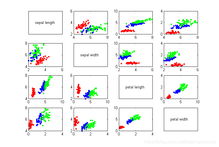
实现的实现过程与 python 的流程是一样的，只是两种编程语言的语法上的差异。

clc
clear all
close all;
load fisheriris;  % 加载数据集
% 数据可视化
x = meas;
y = species;
class = unique(y);
attr = {'sepal length', 'sepal width', 'petal length', 'petal width'};
ind1 = ismember(y, class{1});
ind2 = ismember(y, class{2});
ind3 = ismember(y, class{3});
s=10;
for i=1:4
   for j=1:4
      subplot(4,4,4*(i-1)+j);
      if i==j
          set(gca, 'xtick', [], 'ytick', []);
          text(.2, .5, attr{i});
          set(gca, 'box', 'on');
          continue;
       end
      scatter(x(ind1,i), x(ind1,j), s, 'r', 'MarkerFaceColor', 'r');
      hold on
      scatter(x(ind2,i), x(ind2,j), s, 'b', 'MarkerFaceColor', 'b');
      hold on
      scatter(x(ind3,i), x(ind3,j), s, 'g', 'MarkerFaceColor', 'g');
       set(gca, 'box', 'on');
   end
end
% 随机划分训练集和测试集
ratio = 7/3;
num = length(x);
num_test = round(num/(1+ratio));
num_train = num - num_test;
index = randperm(num);
x_train = x(index(1:num_train),:);
y_train = y(index(1:num_train));
x_test = x(index(num_train+1:end),:);
y_test = y(index(num_train+1:end));
% 构建决策树并预测结果
tree = fitctree(x_train, y_train);
y_test_p = predict(tree, x_test);
% 计算预测准确率
acc = sum(strcmp(y_test,y_test_p))/num_test;
disp(['The accuracy is ', num2str(acc)]);