1.ID3算法
预备知识
1.信息熵:

2.信息增益


算法内容
引入了信息论中的互信息(信息增益)作为选择判别因素的度量,即:以信息增益的下降速度作为选取分类属性的标准,所选的测试属性是从根节点到当前节点的路径上从没有被考虑过的具有最高的信息增益的属性。这就需要计算各个属性的信息增益的值,找出最大的作为判别的属性:
1. 计算先验熵,没有接收到其他的属性值时的平均不确定性,
2. 计算后验墒,在接收到输出符号yi时关于信源的不确定性,
3. 条件熵,对后验熵在输出符号集Y中求期望,接收到全部的付好后对信源的不确定性,
4. 互信息,先验熵和条件熵的差,
实例
是否适合打垒球的决策表如下
| 天气 | 温度 | 湿度 | 风速 | 活动 |
|---|---|---|---|---|
| 晴 | 炎热 | 高 | 弱 | 取消 |
| 晴 | 炎热 | 高 | 强 | 取消 |
| 阴 | 炎热 | 高 | 弱 | 进行 |
| 雨 | 适中 | 高 | 弱 | 进行 |
| 雨 | 寒冷 | 正常 | 弱 | 进行 |
| 雨 | 寒冷 | 正常 | 强 | 取消 |
| 阴 | 寒冷 | 正常 | 强 | 进行 |
| 晴 | 适中 | 高 | 弱 | 取消 |
| 晴 | 寒冷 | 正常 | 弱 | 进行 |
| 雨 | 适中 | 正常 | 弱 | 进行 |
| 晴 | 适中 | 正常 | 强 | 进行 |
| 阴 | 适中 | 高 | 强 | 进行 |
| 阴 | 炎热 | 正常 | 弱 | 进行 |
| 雨 | 适中 | 高 | 强 | 取消 |
1.计算先验熵:在没有接收到其他的任何的属性值时候,活动进行与否的熵根据下表进行计算。

2.分别将各个属性作为决策属性时的条件熵(先计算后验墒,在计算条件熵)
(1) 计算已知天气情况下活动是否进行的条件熵(已知天气情况下对于活动的不确定性)
先计算后验墒:

再计算条件熵:(知道了Y之后,对X的不确定性:知道了天气之后,对活动的不确定性,越小是越好的)
(2)计算已知温度情况时对活动的条件熵(不确定性)
(3)已知湿度情况下对于活动是否进行的条件熵(不确定性)
(4)已知风速情况下对于活动是否进行的条件熵(不确定性)
3.计算信息增益
所以选择天气作为第一个判别因素
在选择了天气作为第一个判别因素之后,我们很容易看出(计算的方法和上面提到的一样),针对上图的中间的三张子表来说,第一张子表在选择湿度作为划分数据的feature的时候,分类问题可以完全解决:湿度正常的情况下进行活动,湿度高的时候取消(在天气状态为晴的条件下);第二个子表不需要划分,即,天气晴的情况下不管其他的因素是什么,活动都要进行;第三张子表当选择风速作为划分的feature时,分类问题也完全解决:风速弱的时候进行,风速强的时候取消(在天气状况为雨的条件下)。


Python实现
import math
import operator

def calcShannonEnt(dataset):
    numEntries = len(dataset)
    labelCounts = {}
    for featVec in dataset:
        currentLabel = featVec[-1]
        if currentLabel not in labelCounts.keys():
            labelCounts[currentLabel] = 0
        labelCounts[currentLabel] +=1

    shannonEnt = 0.0
    for key in labelCounts:
        prob = float(labelCounts[key])/numEntries
        shannonEnt -= prob*math.log(prob, 2)
    return shannonEnt

def CreateDataSet():
    dataset = [[1, 1, 'yes' ],
               [1, 1, 'yes' ],
               [1, 0, 'no'],
               [0, 1, 'no'],
               [0, 1, 'no']]
    labels = ['no surfacing', 'flippers']
    return dataset, labels

def splitDataSet(dataSet, axis, value):
    retDataSet = []
    for featVec in dataSet:
        if featVec[axis] == value:
            reducedFeatVec = featVec[:axis]
            reducedFeatVec.extend(featVec[axis+1:])
            retDataSet.append(reducedFeatVec)

    return retDataSet

def chooseBestFeatureToSplit(dataSet):
    numberFeatures = len(dataSet[0])-1
    baseEntropy = calcShannonEnt(dataSet)
    bestInfoGain = 0.0;
    bestFeature = -1;
    for i in range(numberFeatures):
        featList = [example[i] for example in dataSet]
        uniqueVals = set(featList)
        newEntropy =0.0
        for value in uniqueVals:
            subDataSet = splitDataSet(dataSet, i, value)
            prob = len(subDataSet)/float(len(dataSet))
            newEntropy += prob * calcShannonEnt(subDataSet)
        infoGain = baseEntropy - newEntropy
        if(infoGain > bestInfoGain):
            bestInfoGain = infoGain
            bestFeature = i
    return bestFeature

def majorityCnt(classList):
    classCount ={}
    for vote in classList:
        if vote not in classCount.keys():
            classCount[vote]=0
        classCount[vote]=1
    sortedClassCount = sorted(classCount.iteritems(), key=operator.itemgetter(1), reverse=True)
    return sortedClassCount[0][0]


def createTree(dataSet, labels):
    classList = [example[-1] for example in dataSet]
    if classList.count(classList[0])==len(classList):
        return classList[0]
    if len(dataSet[0])==1:
        return majorityCnt(classList)
    bestFeat = chooseBestFeatureToSplit(dataSet)
    bestFeatLabel = labels[bestFeat]
    myTree = {bestFeatLabel:{}}
    del(labels[bestFeat])
    featValues = [example[bestFeat] for example in dataSet]
    uniqueVals = set(featValues)
    for value in uniqueVals:
        subLabels = labels[:]
        myTree[bestFeatLabel][value] = createTree(splitDataSet(dataSet, bestFeat, value), subLabels)
    return myTree


myDat,labels = CreateDataSet()
createTree(myDat,labels)
Java实现
1.计算给定数据集的香农熵
ID3算法实现中,训练数据和测试数据都是用ArrayList<ArrayList<String>> 存放,每一个子ArrayList是一个sample(feature+label)。即,data中的一列是一个属性,一行是一个样本。
uniqueLabels用来统计不同的label出现的个数。
public double calculateShannonEntropy(ArrayList<ArrayList<String>> data) {
        double shannon = 0.0;

        int length = data.get(0).size(); // length-1就是label的index
        HashMap<String, Integer> uniqueLabels = new HashMap<>();
        for (int i = 0; i < data.size(); i++) {
            if (uniqueLabels.containsKey(data.get(i).get(length - 1))) {
                uniqueLabels.replace(data.get(i).get(length - 1), uniqueLabels.get(data.get(i).get(length - 1)) + 1);
            } else {
                uniqueLabels.put(data.get(i).get(length - 1), 1);
            }
        }
        for (String one : uniqueLabels.keySet()) {
            shannon += -(((double) (uniqueLabels.get(one)) / (data.size()))
                    * Math.log((double) (uniqueLabels.get(one)) / (data.size())) / Math.log(2));
        }
        return shannon;
2 按照给定的feature的取值划分数据集
三个参数(data, index, value)的含义: 将data中第index列上值为value的样本返回,并且在返回的结果中样本不包括index列的特征
public ArrayList<ArrayList<String>> splitDataSetByFeature(ArrayList<ArrayList<String>> data, int index,
            String value) {
        ArrayList<ArrayList<String>> subData = new ArrayList<>();
        for (int i = 0; i < data.size(); i++) {
            ArrayList<String> newSample = new ArrayList<>();
            if (data.get(i).get(index).equals(value)) {
                for (int j = 0; j < data.get(i).size(); j++) {
                    if (j != index) {
                        newSample.add(data.get(i).get(j));
                    }
                }
                subData.add(newSample);
            }
        }
        return subData;
    }
3.选择最好的数据集划分方式
对于一个数据集data,要选择其中的最好的feature来划分数据, 所以需要一列一列(data中的一列是一个属性,一行是一个样本)的比较(比较使用哪个特征来划分得到的信息增益最大)。对于每一列来说,计算该列中的属性值有多少种,然后计算每种属性值的熵的大小,然后按照比例求和。最后比较每一列的熵值的总和,信息增益最大的属性就是我们想要找的最好的属性。
featureStatistic用来统计某一个特征可能的取值以及这些取值的个数
public int chooseBestFeature(ArrayList<ArrayList<String>> data, ArrayList<String> featureName) {
        int featureSize = data.get(0).size();
        int dataSize = data.size();
        int bestFuatrue = -1;
        double bestInfoGain = 0.0;
        double infoGain = 0.0;
        double baseShannon = this.calculateShannonEntropy(data);
        double shannon = 0.0;
        HashMap<String, Integer> featureStatistic = new HashMap<>();
        for (int i = 0; i < featureSize - 1; i++) {
            for (int j = 0; j < data.size(); j++) {
                if (featureStatistic.containsKey(data.get(j).get(i))) {
                    featureStatistic.replace(data.get(j).get(i), featureStatistic.get(data.get(j).get(i)) + 1);
                } else {
                    featureStatistic.put(data.get(j).get(i), 1);
                }
            }

            ArrayList<ArrayList<String>> subdata;
            for (String featureValue : featureStatistic.keySet()) {
                subdata = this.splitDataSetByFeature(data, i, featureValue);
                shannon += this.calculateShannonEntropy(subdata)
                        * ((double) featureStatistic.get(featureValue) / dataSize);
            }
            infoGain = baseShannon - shannon;
            if (infoGain > bestInfoGain) {
                bestInfoGain = infoGain;
                bestFuatrue = i;
            }
            shannon = 0.0;
            featureStatistic.clear();
        }
        return bestFuatrue;
    }
4.构造决策树
递归的构造决策树,注意函数的返回类型是object,而不是DecisionTree(该类的定义下面给出),这是因为当我们构造到叶子结点的时候,我们可能返回的是String(正例还是反例,yes or no,而不再是棵子树),所以使用Object
public Object createDecisionTree(ArrayList<ArrayList<String>> data, ArrayList<String> featureName) {

        int dataSize = data.size();
        int featureSize = data.get(0).size();
        // 如果没有特征了,data.get(0).size = 1 说明只剩下标签了, 开始投票。
        if (data.get(0).size() == 1) {
            return vote(data);
        }
        // 判断是不是所有的sample的label都一致了, 如果是,返回这个统一的类别标签。
        HashSet<String> labels = new HashSet<>();
        for (int i = 0; i < dataSize; i++) {
            if (!labels.contains(data.get(i).get(featureSize - 1))) {
                labels.add(data.get(i).get(featureSize - 1));
            }
        }
        if (labels.size() == 1) {
            return data.get(0).get(featureSize - 1);
        }

        // 选择最好的feature来进行决策树(子决策树)的构建
        int bestFeatureIndex = this.chooseBestFeature(data, featureName);
        String bestFeature = featureName.get(bestFeatureIndex);
        featureName.remove(bestFeatureIndex);

        // 统计上一步选出的最好的属性,都有那些取值。
        HashSet<String> bestFeatureValuesSet = new HashSet<>();
        for (int i = 0; i < data.size(); i++) {
            if (!bestFeatureValuesSet.contains(data.get(i).get(bestFeatureIndex))) {
                bestFeatureValuesSet.add(data.get(i).get(bestFeatureIndex));
            }
        }

        DecisionTree tree = new DecisionTree();
        tree.setAttributeName(bestFeature);

        // 最好的属性的每一个取值,都形成一个子树的root, 开始递归。
        Iterator<String> iterator = bestFeatureValuesSet.iterator();
        while (iterator.hasNext()) {
            ArrayList<String> subFeatureName = new ArrayList<>();
            for (int i = 0; i < featureName.size(); i++) {
                subFeatureName.add(featureName.get(i));
            } // 递归的一个关键问题。
            String featureValue = iterator.next();
            tree.children.put(featureValue,
                    createDecisionTree(splitDataSetByFeature(data, bestFeatureIndex, featureValue), subFeatureName));
        }
        return tree;
    }
5.投票函数
当已经没有属性可以作为划分的依据了, 但是这些样本的类的标签依然不同, 那么这个时候就要投票决定了。这个时候data的形式应该是只有一列标签了。那么我们就找这一列标签中最多的,作为类别返回。
public String vote(ArrayList<ArrayList<String>> data) {
        String voteResult = null;
        int dataSize = data.size();
        int length = data.get(0).size();

        HashMap<String, Integer> sta = new HashMap<>();
        for (int i = 0; i < dataSize; i++) {
            if (!sta.keySet().contains(data.get(i).get(length - 1))) {
                sta.put(data.get(i).get(length - 1), 1);
            } else {
                sta.replace(data.get(i).get(length - 1), sta.get(data.get(i).get(length - 1)) + 1);
            }
        }
        int maxValue = Collections.max(sta.values());
        for (String key : sta.keySet()) {
            if (maxValue == sta.get(key)) {
                voteResult = key;
            }
        }
        return voteResult;
    }
6.决策树的数据结构
不像python中有一个功能比较强大的字典,所以这里自定义了一个决策树的数据结构(类DecisionTree),两个域:
(1)String:用来表示该树(子树)的属性(feature)。
(2) HashMap<String, Object> : key的值表示feature的取值,Object是子树(DecisionTree)或者是最终的label。
典型的一个递归的定义。并且在该类中提供了:
(1)遍历树的方法。
(2)将构造的树输出到指定的文件中。
public class DecisionTree implements Serializable{
    private static final long serialVersionUID = 1L;

    private String attributeName;
    public HashMap<String, Object> children;
    private String decisionTree = "./outputTree/decisionTree.data";

    public void printTree(Object tree, ArrayList<String> record, BufferedWriter bufferedWriter) {
        if (tree instanceof String) {
            record.add((String) tree);
            System.out.println(record);
            try {
                bufferedWriter.write(record.toString());
                bufferedWriter.newLine();
            } catch (IOException e) {
                // TODO Auto-generated catch block
                e.printStackTrace();
            }
            record.remove(record.size() - 1);
            record.remove(record.size() - 1);
            return;
        }
        record.add(((DecisionTree) tree).getAttributeName());
        for (String key : ((DecisionTree) tree).children.keySet()) {
            record.add(key);
            printTree(((DecisionTree) tree).children.get(key), record, bufferedWriter);
        }
        int count = 1;
        while( record.size() > 0 && count <= 2){
            record.remove(record.size() - 1);
            count++;
        }
    }

    public void saveDecisionTree(Object tree)
    {
        try {
            BufferedWriter bufferedWriter = new BufferedWriter(new FileWriter(this.decisionTree));
            this.printTree(tree, new ArrayList<>(), bufferedWriter);
            bufferedWriter.close();
            System.out.println("\r\nthe decision tree has saved in the file: './outputTree/decisionTree.data'");
        } catch (IOException e) {
            // TODO Auto-generated catch block
            e.printStackTrace();
        }
    }
}算法测试和完整代码见:https://blog.csdn.net/robin_Xu_shuai/article/details/74011205
2.C4.5
C4.5是Ross Quinlan在1993年在ID3的基础上改进而提出的。.ID3采用的信息增益度量存在一个缺点,它一般会优先选择有较多属性值的Feature,因为属性值多的Feature会有相对较大的信息增益?(信息增益反映的给定一个条件以后不确定性减少的程度,必然是分得越细的数据集确定性更高,也就是条件熵越小,信息增益越大).为了避免这个不足C4.5中是用信息增益比率(gain ratio)来作为选择分支的准则。信息增益比率通过引入一个被称作分裂信息(Split information)的项来惩罚取值较多的Feature。除此之外,C4.5还弥补了ID3中不能处理特征属性值连续的问题。但是,对连续属性值需要扫描排序,会使C4.5性能下降。
C4.5并不一个算法,而是一组算法—C4.5,非剪枝C4.5和C4.5规则。下图中的算法将给出C4.5的基本工作流程:
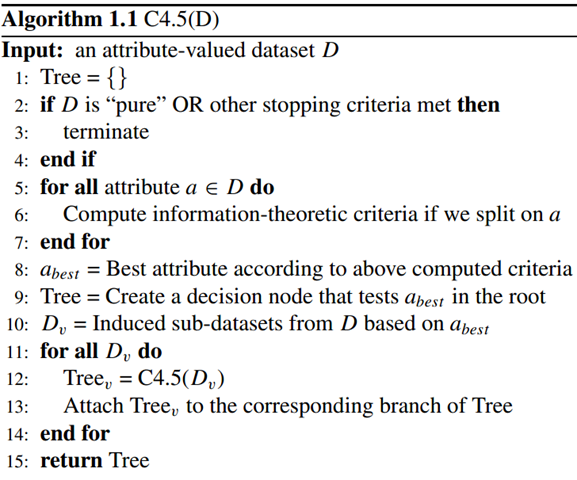
判断对象的属性是有顺序的,属性选择度量又称分裂规则,因为它们决定给定节点上的元组如何分裂。属性选择度量提供了每个属性描述给定训练元组的秩评定,具有最好度量得分的属性被选作给定元组的分裂属性。目前比较流行的属性选择度量有--信息增益、增益率和Gini指标。
在ID3已介绍的关于信息论部分的基础上,介绍信息增益率。
信息增益率使用“分裂信息”值将信息增益规范化。分类信息类似于Info(D),定义如下:
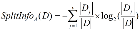
这个值表示通过将训练数据集D划分成对应于属性A测试的v个输出的v个划分产生的信息。信息增益率定义:

选择具有最大增益率的属性作为分裂属性。
建立树类:
package C45Test;

import java.util.ArrayList;
import java.util.List;
import java.util.Map;

public class DecisionTree {

    public TreeNode createDT(List<ArrayList<String>> data,List<String> attributeList){

        System.out.println("当前的DATA为");
        for(int i=0;i<data.size();i++){
            ArrayList<String> temp = data.get(i);
            for(int j=0;j<temp.size();j++){
                System.out.print(temp.get(j)+ " ");
            }
            System.out.println();
        }
        System.out.println("---------------------------------");
        System.out.println("当前的ATTR为");
        for(int i=0;i<attributeList.size();i++){
            System.out.print(attributeList.get(i)+ " ");
        }
        System.out.println();
        System.out.println("---------------------------------");
        TreeNode node = new TreeNode();
        String result = InfoGain.IsPure(InfoGain.getTarget(data));
        if(result != null){
            node.setNodeName("leafNode");
            node.setTargetFunValue(result);
            return node;
        }
        if(attributeList.size() == 0){
            node.setTargetFunValue(result);
            return node;
        }else{
            InfoGain gain = new InfoGain(data,attributeList);
            double maxGain = 0.0;
            int attrIndex = -1;
            for(int i=0;i<attributeList.size();i++){
                double tempGain = gain.getGainRatio(i);
                if(maxGain < tempGain){
                    maxGain = tempGain;
                    attrIndex = i;
                }
            }
            System.out.println("选择出的最大增益率属性为: " + attributeList.get(attrIndex));
            node.setAttributeValue(attributeList.get(attrIndex));
            List<ArrayList<String>> resultData = null;
            Map<String,Long> attrvalueMap = gain.getAttributeValue(attrIndex);
            for(Map.Entry<String, Long> entry : attrvalueMap.entrySet()){
                resultData = gain.getData4Value(entry.getKey(), attrIndex);
                TreeNode leafNode = null;
                System.out.println("当前为"+attributeList.get(attrIndex)+"的"+entry.getKey()+"分支。");
                if(resultData.size() == 0){
                    leafNode = new TreeNode();
                    leafNode.setNodeName(attributeList.get(attrIndex));
                    leafNode.setTargetFunValue(result);
                    leafNode.setAttributeValue(entry.getKey());
                }else{
                    for (int j = 0; j < resultData.size(); j++) {
                        resultData.get(j).remove(attrIndex);
                    }
                    ArrayList<String> resultAttr = new ArrayList<String>(attributeList);
                    resultAttr.remove(attrIndex);
                    leafNode = createDT(resultData,resultAttr);
                }
                node.getChildTreeNode().add(leafNode);
                node.getPathName().add(entry.getKey());
            }
        }
        return node;
    }

    class TreeNode{

        private String attributeValue;
        private List<TreeNode> childTreeNode;
        private List<String> pathName;
        private String targetFunValue;
        private String nodeName;

        public TreeNode(String nodeName){

            this.nodeName = nodeName;
            this.childTreeNode = new ArrayList<TreeNode>();
            this.pathName = new ArrayList<String>();
        }

        public TreeNode(){
            this.childTreeNode = new ArrayList<TreeNode>();
            this.pathName = new ArrayList<String>();
        }

        public String getAttributeValue() {
            return attributeValue;
        }

        public void setAttributeValue(String attributeValue) {
            this.attributeValue = attributeValue;
        }

        public List<TreeNode> getChildTreeNode() {
            return childTreeNode;
        }

        public void setChildTreeNode(List<TreeNode> childTreeNode) {
            this.childTreeNode = childTreeNode;
        }

        public String getTargetFunValue() {
            return targetFunValue;
        }

        public void setTargetFunValue(String targetFunValue) {
            this.targetFunValue = targetFunValue;
        }

        public String getNodeName() {
            return nodeName;
        }

        public void setNodeName(String nodeName) {
            this.nodeName = nodeName;
        }

        public List<String> getPathName() {
            return pathName;
        }

        public void setPathName(List<String> pathName) {
            this.pathName = pathName;
        }

    }
}
增益率计算类
package C45Test;

import java.util.ArrayList;
import java.util.HashMap;
import java.util.HashSet;
import java.util.Iterator;
import java.util.List;
import java.util.Map;
import java.util.Set;

//C 4.5 实现
public class InfoGain {

    private List<ArrayList<String>> data;
    private List<String> attribute;

    public InfoGain(List<ArrayList<String>> data,List<String> attribute){

        this.data = new ArrayList<ArrayList<String>>();
        for(int i=0;i<data.size();i++){
            List<String> temp = data.get(i);
            ArrayList<String> t = new ArrayList<String>();
            for(int j=0;j<temp.size();j++){
                t.add(temp.get(j));
            }
            this.data.add(t);
        }

        this.attribute = new ArrayList<String>();
        for(int k=0;k<attribute.size();k++){
            this.attribute.add(attribute.get(k));
        }
        /*this.data = data;
        this.attribute = attribute;*/
    }

    //获得熵
    public double getEntropy(){

        Map<String,Long> targetValueMap = getTargetValue();
        Set<String> targetkey = targetValueMap.keySet();
        double entropy = 0.0;
        for(String key : targetkey){
            double p = MathUtils.div((double)targetValueMap.get(key), (double)data.size());
            entropy += (-1) * p * Math.log(p);
        }
        return entropy;
    }

    //获得InfoA
    public double getInfoAttribute(int attributeIndex){

        Map<String,Long> attributeValueMap = getAttributeValue(attributeIndex);
        double infoA = 0.0;
        for(Map.Entry<String, Long> entry : attributeValueMap.entrySet()){
            int size = data.size();
            double attributeP = MathUtils.div((double)entry.getValue() , (double) size);
            Map<String,Long> targetValueMap = getAttributeValueTargetValue(entry.getKey(),attributeIndex);
            long totalCount = 0L;
            for(Map.Entry<String, Long> entryValue :targetValueMap.entrySet()){
                totalCount += entryValue.getValue();
            }
            double valueSum = 0.0;
            for(Map.Entry<String, Long> entryTargetValue : targetValueMap.entrySet()){
                 double p = MathUtils.div((double)entryTargetValue.getValue(), (double)totalCount);
                 valueSum += Math.log(p) * p;
            }
            infoA += (-1) * attributeP * valueSum;
        }
        return infoA;

    }

    //得到属性值在决策空间的比例
    public Map<String,Long> getAttributeValueTargetValue(String attributeName,int attributeIndex){

        Map<String,Long> targetValueMap = new HashMap<String,Long>();
        Iterator<ArrayList<String>> iterator = data.iterator();
        while(iterator.hasNext()){
            List<String> tempList = iterator.next();
            if(attributeName.equalsIgnoreCase(tempList.get(attributeIndex))){
                int size = tempList.size();
                String key = tempList.get(size - 1);
                Long value = targetValueMap.get(key);
                targetValueMap.put(key, value != null ? ++value :1L);
            }
        }
        return targetValueMap;
    }

    //得到属性在决策空间上的数量
    public Map<String,Long> getAttributeValue(int attributeIndex){

        Map<String,Long> attributeValueMap = new HashMap<String,Long>();
        for(ArrayList<String> note : data){
            String key = note.get(attributeIndex);
            Long value = attributeValueMap.get(key);
            attributeValueMap.put(key, value != null ? ++value :1L);
        }
        return attributeValueMap;

    }

    public List<ArrayList<String>> getData4Value(String attrValue,int attrIndex){

        List<ArrayList<String>> resultData = new ArrayList<ArrayList<String>>();
        Iterator<ArrayList<String>> iterator = data.iterator();
        for(;iterator.hasNext();){
            ArrayList<String> templist = iterator.next();
            if(templist.get(attrIndex).equalsIgnoreCase(attrValue)){
                ArrayList<String> temp = (ArrayList<String>) templist.clone();
                resultData.add(temp);
            }
        }
        return resultData;
    }

    //获得增益率
    public double getGainRatio(int attributeIndex){
        return MathUtils.div(getGain(attributeIndex), getSplitInfo(attributeIndex));
    }

    //获得增益量
    public double getGain(int attributeIndex){
        return getEntropy() - getInfoAttribute(attributeIndex);
    }

    //得到惩罚因子
    public double getSplitInfo(int attributeIndex){

        Map<String,Long> attributeValueMap = getAttributeValue(attributeIndex);
        double splitA = 0.0;
        for(Map.Entry<String, Long> entry : attributeValueMap.entrySet()){
            int size = data.size();
            double attributeP = MathUtils.div((double)entry.getValue() , (double) size);
            splitA += attributeP * Math.log(attributeP) * (-1);
        }
        return splitA;
    }

    //得到目标函数在当前集合范围内的离散的值
    public Map<String,Long> getTargetValue(){

        Map<String,Long> targetValueMap = new HashMap<String,Long>();
        Iterator<ArrayList<String>> iterator = data.iterator();
        while(iterator.hasNext()){
            List<String> tempList = iterator.next();
            String key = tempList.get(tempList.size() - 1);
            Long value = targetValueMap.get(key);
            targetValueMap.put(key, value != null ? ++value : 1L);
        }
        return targetValueMap;
    }

    //获得TARGET值
    public static List<String> getTarget(List<ArrayList<String>> data){

        List<String> list = new ArrayList<String>();
        for(ArrayList<String> temp : data){
            int index = temp.size() -1;
            String value = temp.get(index);
            list.add(value);
        }
        return list;
    }

    //判断当前纯度是否100%
    public static String IsPure(List<String> list){

        Set<String> set = new HashSet<String>();
        for(String name :list){
            set.add(name);
        }
        if(set.size() > 1) return null;
        Iterator<String> iterator = set.iterator();
        return iterator.next();
    }


}
测试类,数据集读取以上的分别放到2个List中。
package C45Test;

import java.util.ArrayList;
import java.util.List;

import C45Test.DecisionTree.TreeNode;

public class MainC45 {

    private static final List<ArrayList<String>> dataList = new ArrayList<ArrayList<String>>();
    private static final List<String> attributeList = new ArrayList<String>();

    public static void main(String args[]){

        DecisionTree dt = new DecisionTree();
        TreeNode node = dt.createDT(configData(),configAttribute());
        System.out.println();
    }
}
大数运算工具类
package C45Test;
import java.math.BigDecimal;

public abstract class MathUtils {

    //默认余数长度
    private static final int DIV_SCALE = 10;

    //受限于DOUBLE长度
    public static double add(double value1,double value2){

        BigDecimal big1 = new BigDecimal(String.valueOf(value1));
        BigDecimal big2 = new BigDecimal(String.valueOf(value2));
        return big1.add(big2).doubleValue();
    }

    //大数加法
    public static double add(String value1,String value2){

        BigDecimal big1 = new BigDecimal(value1);
        BigDecimal big2 = new BigDecimal(value2);
        return big1.add(big2).doubleValue();
    }

    public static double div(double value1,double value2){

        BigDecimal big1 = new BigDecimal(String.valueOf(value1));
        BigDecimal big2 = new BigDecimal(String.valueOf(value2));
        return big1.divide(big2,DIV_SCALE,BigDecimal.ROUND_HALF_UP).doubleValue();
    }

    public static double mul(double value1,double value2){

        BigDecimal big1 = new BigDecimal(String.valueOf(value1));
        BigDecimal big2 = new BigDecimal(String.valueOf(value2));
        return big1.multiply(big2).doubleValue();
    }

    public static double sub(double value1,double value2){

        BigDecimal big1 = new BigDecimal(String.valueOf(value1));
        BigDecimal big2 = new BigDecimal(String.valueOf(value2));
        return big1.subtract(big2).doubleValue();
    }

    public static double returnMax(double value1, double value2) {

        BigDecimal big1 = new BigDecimal(value1);
        BigDecimal big2 = new BigDecimal(value2);
        return big1.max(big2).doubleValue();
    }
}
3.CART算法
原理:
分类回归树算法:CART(Classification And Regression Tree)算法采用一种二分递归分割的技术,将当前的样本集分为两个子样本集,使得生成的的每个非叶子节点都有两个分支。因此,CART算法生成的决策树是结构简洁的二叉树。
分类树两个基本思想:第一个是将训练样本进行递归地划分自变量空间进行建树的想法,第二个想法是用验证数据进行剪枝。
建树:在分类回归树中,我们把类别集Result表示因变量,选取的属性集attributelist表示自变量,通过递归的方式把attributelist把p维空间划分为不重叠的矩形,具体建树的基本步骤参见:http://baike.baidu.com/view/3075445.htm。
CART算法是怎样进行样本划分的呢?它检查每个变量和该变量所有可能的划分值来发现最好的划分,对离散值如{x,y,x},则在该属性上的划分有三种情况({{x,y},{z}},{{x,z},y},{{y,z},x}),空集和全集的划分除外;对于连续值处理引进“分裂点”的思想,假设样本集中某个属性共n个连续值,则有n-1个分裂点,每个“分裂点”为相邻两个连续值的均值 (a[i] + a[i+1]) / 2。将每个属性的所有划分按照他们能减少的杂质(合成物中的异质,不同成分)量来进行排序,杂质的减少被定义为划分前的杂质减去划分之后每个节点的杂质量*划分所占样本比率之和,目前最流行的杂质度量方法是:GINI指标,如果我们用k,k=1,2,3……C表示类,其中C是类别集Result的因变量数目,一个节点A的GINI不纯度定义为:

其中,Pk表示观测点中属于k类得概率,当Gini(A)=0时所有样本属于同一类,当所有类在节点中以相同的概率出现时,Gini(A)最大化,此时值为(C-1)C/2。
对于分类回归树,A如果它不满足“T都属于同一类别or T中只剩下一个样本”,则此节点为非叶节点,所以尝试根据样本的每一个属性及可能的属性值,对样本的进行二元划分,假设分类后A分为B和C,其中B占A中样本的比例为p,C为q(显然p+q=1)。则杂质改变量:Gini(A) -p*Gini(B)-q*Gini(C),每次划分该值应为非负,只有这样划分才有意义,对每个属性值尝试划分的目的就是找到杂质该变量最大的一个划分,该属性值划分子树即为最优分支。
剪枝:在CART过程中第二个关键的思想是用独立的验证数据集对训练集生长的树进行剪枝。
分析分类回归树的递归建树过程,不难发现它实质上存在着一个数据过度拟合问题。在决策树构造时,由于训练数据中的噪音或孤立点,许多分枝反映的是训练数据中的异常,使用这样的判定树对类别未知的数据进行分类,分类的准确性不高。因此试图检测和减去这样的分支,检测和减去这些分支的过程被称为树剪枝。树剪枝方法用于处理过分适应数据问题。通常,这种方法使用统计度量,减去最不可靠的分支,这将导致较快的分类,提高树独立于训练数据正确分类的能力。
决策树常用的剪枝常用的简直方法有两种:事前剪枝和事后剪枝,CART算法经常采用事后剪枝方法:该方法是通过在完全生长的树上剪去分枝实现的,通过删除节点的分支来剪去树节点。最下面未被剪枝的节点成为树叶。
CART用的成本复杂性标准是分类树的简单误分(基于验证数据的)加上一个对树的大小的惩罚因素。惩罚因素是有参数的,我们用a表示,每个节点的惩罚。成本复杂性标准对于一个数来说是Err(T)+a|L(T)|,其中Err(T)是验证数据被树误分部分,L(T)是树T的叶节点树,a是每个节点的惩罚成本:一个从0向上变动的数字。当a=0对树有太多的节点没有惩罚,用的成本复杂性标准是完全生长的没有剪枝的树。在剪枝形成的一系列树中,从其中选择一个在验证数据集上具有最小误分的树是很自然的,我们把这个树成为最小误分树。
算法实现:
本文根据一个样本集,进行了CART算法的简单实现。该样本集中每个样本有十六个特征属性和一个结果属性,为了降低划分的难度,每个特征属性取两个不同的离散值,结果属性有两个离散值:Yes和No。
数据结构定义:在该算法中定义了三种数据结构:存储样本属性名称及取值的Node属性,存储单个样本的EXampleSet属性,树的节点属性dataNode;存放在DataStructure.h中,代码如下:
typedef struct tagNode
{//存储属性
	string name;//属性的名称
	string value;//属性取值
}Node;
typedef struct tagExampleSet
{//样本存储
	string example[16];//样本的每个属性上的属性值
	string decision;//样本的结果类
}ExampleSet;
typedef struct Data_Node{
	//节点的数据结构,结果分为两类yes类和No类
	int Yesnum;//类yes得样本数目
	int Nonum;//类no得样本数
	vector<ExampleSet> myVector;//存储样本
	Data_Node *LeftNode;//左子树
	Data_Node *RightNode;//右子树
	int Property;//划分选取的属性
	string Proper_value;//所选的属性的值
	int nodenum;//标示节点
	bool leavenode;//标示叶节点
}dataNode;
样本读取及处理:用两个文件分别存储样本的属性及所有样本。文件t存储样本的十六个自变量属性、类别属性的名称和离散值集合,文件t1是所有样本的集合,用ReadFile类读取文件,并把它们分别存储在两个向量中。建树的过程在MySufan类中,该类地方法列表如下:
MySuanfa();
	~MySuanfa();
	void Method();//调用建树、剪枝方法
	void BuildTree(Data_Node*thisNode);//建树方法,每次调用DeviceTree对非叶节点进行划分
	void DeviceTree(Data_Node*thisNode,int i);//对非叶结点进行划分,分出左节点,有节点
	int Choose_Property(Data_Node* thisNode);//返回选择的属性值
	double pure(int i1,int i2,int i3);//纯度计算函数,每次计算最优划分时用
	void Deal(Data_Node* d);//剪枝函数,此函数对建好的树用测试样本进行剪枝
	void levelorder(Data_Node * p);//层次遍历,此方法按曾给决策点分配序号,用于剪枝
	void inorder(Data_Node *p);//中序遍历,和建树的前序遍历用于确定树的结构
	void BuildTest(Data_Node *d,int t);//此方法用于计算当取不同决策点时,建树样本的错误样本数,t为决策点数目
	void CutTree(Data_Node *d,int k,int t);//k为单个样本,t为决策点数,根据决策点对测试样本集进行测试
	void ClassOfNode(vector<ExampleSet>);//本方法用于切割原始样本集,将样本分为测试样本和建树样本
递归建树:建树按照递归方式进行建树,采用全部样本的2/3进行建树,首先找到一个划分值,如果不存在返回-1,然后判断一个树是否为叶子节点,不为叶子节点按照划分值进行划分,关键代码如下:
void MySuanfa::BuildTree(Data_Node* thisNode)
{
	 if(thisNode!=NULL){// //节点不为空
       nodenum++;
		 thisNode->nodenum=nodenum;
       int getProperty=Choose_Property(thisNode);//找到划分
		 thisNode->Property=getProperty;
if((thisNode->Yesnum*thisNode->Nonum==0)||getProperty==-1)
		 {//如果划分为-1,则无法再次划分
			 thisNode->Property=-1;
			 thisNode->leavenode=true;
		}
	     else
		 {//递归建树
          thisNode->leavenode=false;
			 DeviceTree(thisNode,getProperty);//将父节点按照划分属性进行划分
		    BuildTree(thisNode->LeftNode);//递归建立左子树
           BuildTree(thisNode->RightNode);//递归建立右子树
		 }
	 }
}
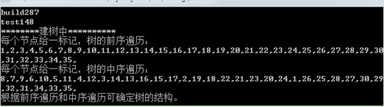
分析上面代码,Choose_Property(thisNode);函数的作用是将thisNode中的样本尝试进行最优划分,划分的依据就是杂质最大该变量,如果划分成功返回属性下标,否则返回-1,我们在样本中每个属性默认取两个离散值。注意到方法中对书中定义的leavenode和nodenum两个变量的操作,他们的用途是什么呢?nodenum的第一个作用是树的遍历,将每一个节点赋予一个唯一的值,建树的过程是前序建树,建树结束后根据树的中序遍历可以唯一确定树的结构,nodenum的第二个作用和leavenode的作用将会在剪枝过程中用到,后面将会提到。
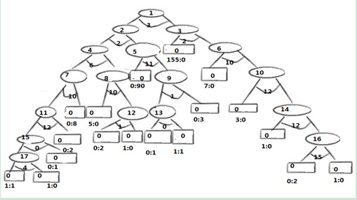
当建树结束后,树的前序即为nodenum从小到大的排序,然后通过调用中序遍历函数输出树的中序序列,确定树的结构。该树含有17个决策点(非叶子节点),18个叶子节点。
树中决策点的划分代码对应的属性名称:
0————handicapped-infants ; 1————water-project-cost-sharing
2————adoption-of-the-budget-resolution ; 3————physician-fee-freeze
4————el-salvador-aid ; 5————religious-groups-in-schools
6————anti-satellite-test-ban; 7————aid-to-nicaraguan-contras
8————mx-missile ; 9————immigration
10————synfuels-corporation-cutback ; 11————education-spending
12————superfund-right-to-sue ; 13————crime
14————duty-free-exports ; 15—export-administration-act-south-africa
按照递归分类的算法,最终生成的树的叶子节点中或者同属一类或者只有一个样本,分析树的结构我们可以发现,有两个叶子节点8和23不符合这种情况,却成了叶子节点。这与所选样本有关,在这两个叶节点中两个样本的十六个特征属性值都相同,只有所属类别不同,所以无法根据递归算法进行分类。另当选取physician-fee-freeze 和adoption-of-the-budget-resolution两种属性进行决策时,样本所属的类别已经基本判定,造成这种情况我们可认为这两种属性在样本中所占的权重很大,只要确定这两种情况,树的大部分样本的分类就已确定。
剪枝:用训练样本建树结束后,就是进行树的剪枝阶段,本算法采用样本集的后1/3作为测试进行剪枝。
树的决策点:如果一个节点为非叶节点,则称该节点为一个树的决策点。树的剪枝就是减去过分拟合给树带来的的冗余,用尽可能少的决策点、尽可能低的树高获取尽可能大的正确率。
如何获取树的决策点?逐层确定树的决策点,并根据决策点数目进行剪枝是剪枝的关键。
根据二叉树的特性可知树的非叶节点=叶节点-1;所以可以从树的节点数中得知树种非叶结点的数量。本程序根据这一特性将树的决策点逐层赋值,根节点赋值1,根节点的左节点赋值2……,这一过程通过层次遍历实现。并将该值赋给nodenum,对于叶子节点nodenum为0关键代码如下:
void MySuanfa::levelorder(Data_Node* p)
{
	int node=1;
    list<Data_Node *>q;
    if(p)q.push_back(p);
	p->nodenum=node;
 while(!q.empty())
    {
       	p=q.front();
        q.pop_front();
        if(p->LeftNode)
		{
			if(p->LeftNode->leavenode)
			{//如果该节点的左节点是子节点,则将nodenum赋0
             p->LeftNode->nodenum=0;
			}
			else
			{//否则将该节点赋一个node值,该值表示此决策点的顺序
			node++;
			p->LeftNode->nodenum=node;
			q.push_back(p->LeftNode);
			}
		}
        if(p->RightNode)
		{
			if(p->RightNode->leavenode)//
			{//如果该节点的右节点是子节点,则将nodenum赋0
				 p->RightNode->nodenum=0;
			}
			else
			{//否则将该节点赋一个node值,该值表示此决策点的顺序
				node++;
			p->RightNode->nodenum=node;
			q.push_back(p->RightNode);
			}
		}
}
}
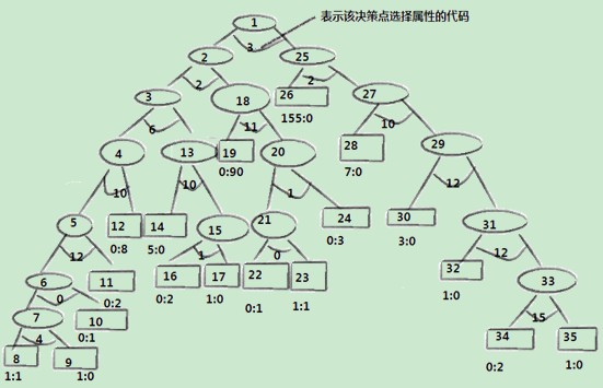
遍历结束后,每一个决策点数目可以确定一个树,我们就可以根据树的决策点数对训练样本和测试样本的误差进行统计,怎样根据决策点数确定树的结构?可以将树的前序遍历进行改进,对于t个决策点,节点为0或大于t的都是叶子节点,一旦确定叶子节点,树的结构就清楚了,下图为重新赋值后的树,在该图中,如当有3个决策点时,2的子节点和3的子节点都是叶子节点,当用改进的前序遍历便立时会输出有3个决策点:(1,2,3);4个叶子节点(4,5,0,6)的子树:
不同决策点可对应不同子树,通过前序遍历可以将叶子节点中的错误样本统计出来计算该树情况下错误样本的个数,然后再用测试样本遍历树,统计测试样本再改树下错误样本个数最后得出结果集如下:
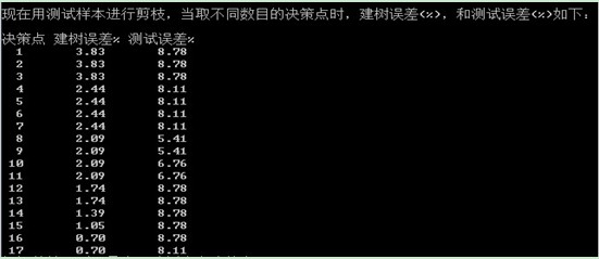
通过比较可知当树有8和9个决策点时,测试误差最小,我们取8,因为此时树比9个决策点简单,我们取含有8个决策点为最小误分树。最小误分树结构如下:
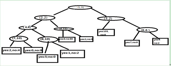
上图中最小误分树非叶节点中的两个值,第一个表示决策点表示,第二个表示选择的属性的代码,叶子节点中两数表示每一类的数目。
我们定义最优剪枝的方法是在剪枝序列中含有误差在最小误差树的一个标准差之内的最小树,算出的最小误差率被砍做一个带有标准差等于的随机变量的观测值,其中Emin对最小误差树的错误率,Nval是验证集的个数:Emin=5.41%,Nval=148,所以到当树有4个决策点时,为最优剪枝。

参考:
1.https://blog.csdn.net/robin_Xu_shuai/article/details/74011205
2.https://blog.csdn.net/qq_36330643/article/details/77415451
3.https://www.cnblogs.com/yjd_hycf_space/p/6940068.html
4.https://www.cnblogs.com/sumuncle/p/5610877.html