吉吉:
import numpy as np
import pandas as pd
df = pd.read_csv('iris.data')
df.head()
df.columns=['sepal_len', 'sepal_wid', 'petal_len', 'petal_wid', 'class']
df.head()# split data table into data X and class labels y
X = df.iloc[:,0:4].values
y = df.iloc[:,4].values
from matplotlib import pyplot as plt
import math
label_dict = {1: 'Iris-Setosa',
2: 'Iris-Versicolor',
3: 'Iris-Virgnica'}
feature_dict = {0: 'sepal length [cm]',
1: 'sepal width [cm]',
2: 'petal length [cm]',
3: 'petal width [cm]'}
plt.figure(figsize=(8, 6))
for cnt in range(4):
plt.subplot(2, 2, cnt+1)
for lab in ('Iris-setosa', 'Iris-versicolor', 'Iris-virginica'):
plt.hist(X[y==lab, cnt],
label=lab,
bins=10,
alpha=0.3,)
plt.xlabel(feature_dict[cnt])
plt.legend(loc='upper right', fancybox=True, fontsize=8)
plt.tight_layout()
plt.show()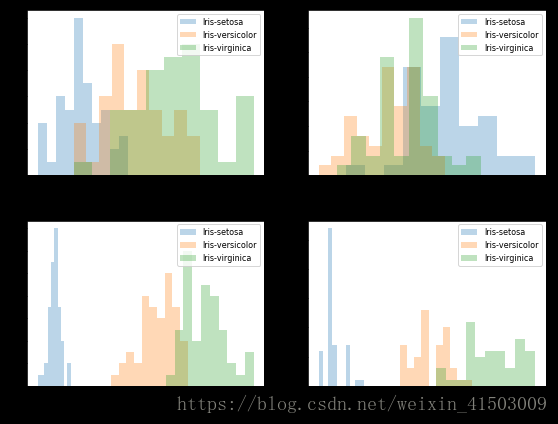
from sklearn.preprocessing import StandardScaler
X_std = StandardScaler().fit_transform(X)
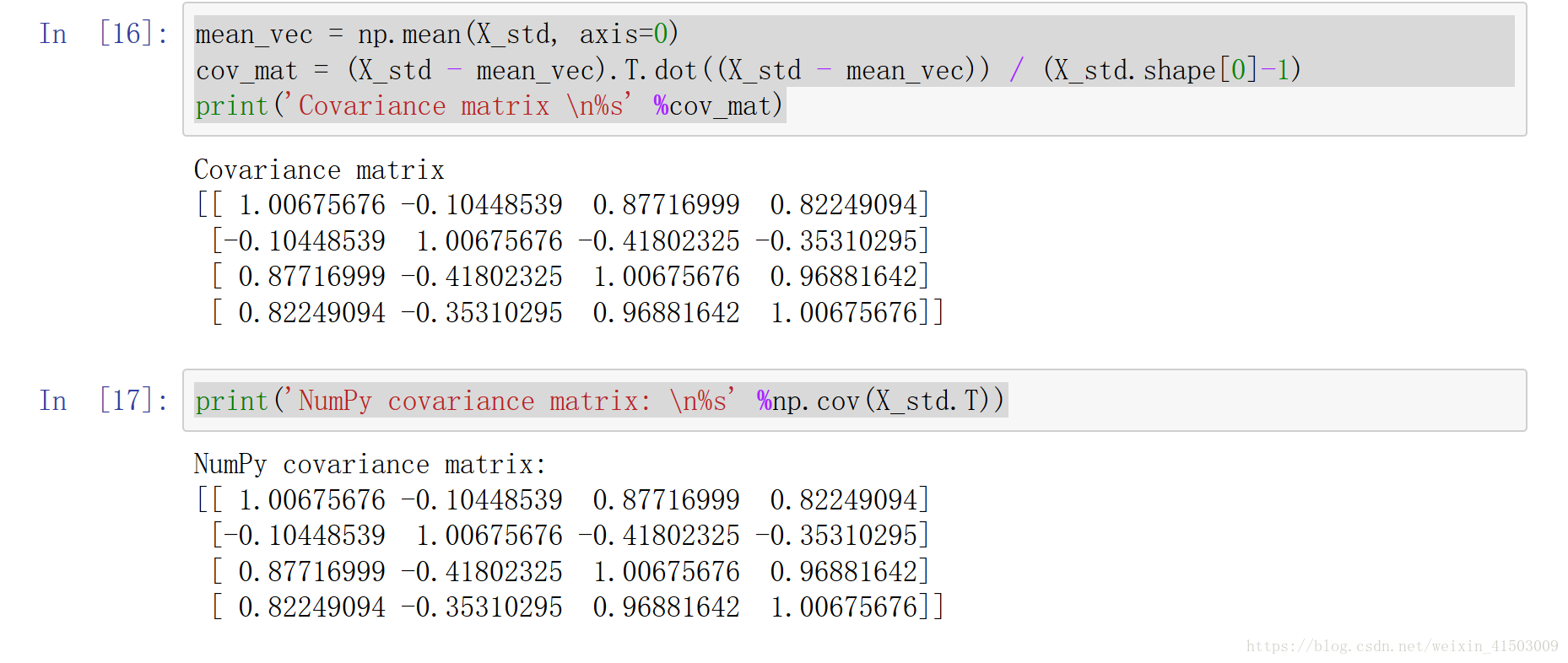
print (X_std)mean_vec = np.mean(X_std, axis=0)
cov_mat = (X_std - mean_vec).T.dot((X_std - mean_vec)) / (X_std.shape[0]-1)
print('Covariance matrix \n%s' %cov_mat)
print('NumPy covariance matrix: \n%s' %np.cov(X_std.T))
cov_mat = np.cov(X_std.T)

eig_vals, eig_vecs = np.linalg.eig(cov_mat)

print('Eigenvectors \n%s' %eig_vecs)
print('\nEigenvalues \n%s' %eig_vals)
Eigenvectors
[[ 0.52308496 -0.36956962 -0.72154279 0.26301409]
[-0.25956935 -0.92681168 0.2411952 -0.12437342]
[ 0.58184289 -0.01912775 0.13962963 -0.80099722]
[ 0.56609604 -0.06381646 0.63380158 0.52321917]]
Eigenvalues
[2.92442837 0.93215233 0.14946373 0.02098259]
# Make a list of (eigenvalue, eigenvector) tuples
eig_pairs = [(np.abs(eig_vals[i]), eig_vecs[:,i]) for i in range(len(eig_vals))]
print (eig_pairs)
print ('----------')
# Sort the (eigenvalue, eigenvector) tuples from high to low
eig_pairs.sort(key=lambda x: x[0], reverse=True)

# Visually confirm that the list is correctly sorted by decreasing eigenvalues
print('Eigenvalues in descending order:')
for i in eig_pairs:
    print(i[0])
[(2.9244283691111144, array([ 0.52308496, -0.25956935, 0.58184289, 0.56609604])), (0.9321523302535064, array([-0.36956962, -0.92681168, -0.01912775, -0.06381646])), (0.14946373489813314, array([-0.72154279, 0.2411952 , 0.13962963, 0.63380158])), (0.020982592764270606, array([ 0.26301409, -0.12437342, -0.80099722, 0.52321917]))]
----------
Eigenvalues in descending order:
2.9244283691111144
0.9321523302535064
0.14946373489813314
0.020982592764270606tot = sum(eig_vals)
var_exp = [(i / tot)*100 for i in sorted(eig_vals, reverse=True)]
print (var_exp)
cum_var_exp = np.cumsum(var_exp)
cum_var_exp[72.62003332692034, 23.147406858644135, 3.7115155645845164, 0.5210442498510154]
array([ 72.62003333, 95.76744019, 99.47895575, 100. ])a = np.array([1,2,3,4])
print (a)
print ('-----------')
print (np.cumsum(a))[1 2 3 4]
-----------
[ 1 3 6 10]
plt.figure(figsize=(6, 4))

plt.bar(range(4), var_exp, alpha=0.5, align='center',
            label='individual explained variance')
plt.step(range(4), cum_var_exp, where='mid',
             label='cumulative explained variance')
plt.ylabel('Explained variance ratio')
plt.xlabel('Principal components')
plt.legend(loc='best')
plt.tight_layout()
plt.show()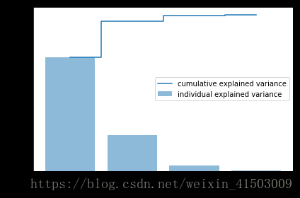
matrix_w = np.hstack((eig_pairs[0][1].reshape(4,1),
                      eig_pairs[1][1].reshape(4,1)))

print('Matrix W:\n', matrix_w)
Y = X_std.dot(matrix_w)
Y
plt.figure(figsize=(6, 4))
for lab, col in zip(('Iris-setosa', 'Iris-versicolor', 'Iris-virginica'),
('blue', 'red', 'green')):
plt.scatter(X[y==lab, 0],
X[y==lab, 1],
label=lab,
c=col)
plt.xlabel('sepal_len')
plt.ylabel('sepal_wid')
plt.legend(loc='best')
plt.tight_layout()
plt.show()

plt.figure(figsize=(6, 4))
for lab, col in zip(('Iris-setosa', 'Iris-versicolor', 'Iris-virginica'),
                        ('blue', 'red', 'green')):
     plt.scatter(Y[y==lab, 0],
                Y[y==lab, 1],
                label=lab,
                c=col)
plt.xlabel('Principal Component 1')
plt.ylabel('Principal Component 2')
# plt.legend(loc='lower center')
plt.legend(loc='best')
plt.tight_layout()
plt.show()

数据集来源:https://download.csdn.net/download/weixin_41503009/10683513
当然也可以从sklearn导入数据集,我仅仅想赚几个C币,哈哈哈咯。。。。。。。。