KNN算法实现图像分类

首先，回顾k-Nearest Neighbor（k-NN）分类器，可以说是最简单易懂的机器学习算法。 实际上，k-NN非常简单，根本不会执行任何“学习”，以及介绍k-NN分类器的工作原理。 然后，我们将k-NN应用于Kaggle Dogs vs. Cats数据集，这是Microsoft的Asirra数据集的一个子集。顾名思义，Dogs vs. Cats数据集的目标是对给定图像是否包含狗或猫进行分类。 

Kaggle Dogs vs. Cats dataset

---

Dogs vs. Cats数据集实际上是几年前Kaggle挑战的一部分。 挑战本身很简单：给出一个图像，预测它是否包含一只狗或一只猫：

建立的工程文件的结构

k-NN classifier for image classificationShell

$ tree --filelimit 10
.
├── kaggle_dogs_vs_cats
│   └── train [25000 entries exceeds filelimit, not opening dir]
└── knn_classifier.py

2 directories, 1 file

k-Nearest Neighbor分类器是迄今为止最简单的机器学习/图像分类算法。 事实上，它很简单，实际上并没有“学习”任何东西。

在内部，该算法仅依赖于特征向量之间的距离，就像构建图像搜索引擎一样 - 只是这次，我们有与每个图像相关联的标签，因此我们可以预测并返回图像的实际类别。

简而言之，k-NN算法通过找到k个最接近的例子中最常见的类来对未知数据点进行分类。 k个最近的例子中的每个数据点都投了一票，而得票最多的类别获胜！

或者，用简单的英语：“告诉我你的邻居是谁，我会告诉你你是谁”。

在这里我们可以看到有两类图像，并且每个相应类别中的每个数据点在n维空间中相对靠近地分组。 我们的狗往往有深色的外套，不是很蓬松，而我们的猫有非常轻的外套非常蓬松。

这意味着红色圆圈中两个数据点之间的距离远小于红色圆圈中的数据点与蓝色圆圈中的数据点之间的距离。

为了应用k-最近邻分类，我们需要定义距离度量或相似度函数。 常见的选择包括欧几里德距离（差值平方和）、曼哈顿距离（绝对值距离）。可以根据数据类型使用其他距离度量/相似度函数（卡方距离通常用于分布即直方图）。 在今天的博客文章中，为了简单起见，我们将使用欧几里德距离来比较图像的相似性。

扫描二维码关注公众号，回复： 4052012 查看本文章

建立knn.py

# import the necessary packages
from sklearn.neighbors import KNeighborsClassifier
from sklearn.model_selection import train_test_split
from imutils import paths
import numpy as np
import argparse
import imutils
import cv2
import os

def image_to_feature_vector(image, size=(32, 32)):
	# resize the image to a fixed size, then flatten the image into
	# a list of raw pixel intensities
	return cv2.resize(image, size).flatten()

def extract_color_histogram(image, bins=(8, 8, 8)):
	# extract a 3D color histogram from the HSV color space using
	# the supplied number of `bins` per channel
	hsv = cv2.cvtColor(image, cv2.COLOR_BGR2HSV)
	hist = cv2.calcHist([hsv], [0, 1, 2], None, bins,
		[0, 180, 0, 256, 0, 256])
 
	# handle normalizing the histogram if we are using OpenCV 2.4.X
	if imutils.is_cv2():
		hist = cv2.normalize(hist)
 
	# otherwise, perform "in place" normalization in OpenCV 3 (I
	# personally hate the way this is done
	else:
		cv2.normalize(hist, hist)
 
	# return the flattened histogram as the feature vector
	return hist.flatten()

# construct the argument parse and parse the arguments
ap = argparse.ArgumentParser()
ap.add_argument("-d", "--dataset", required=True,
	help="path to input dataset")
ap.add_argument("-k", "--neighbors", type=int, default=1,
	help="# of nearest neighbors for classification")
ap.add_argument("-j", "--jobs", type=int, default=-1,
	help="# of jobs for k-NN distance (-1 uses all available cores)")
args = vars(ap.parse_args())

# grab the list of images that we'll be describing
print("[INFO] describing images...")
imagePaths = list(paths.list_images(args["dataset"]))
 
# initialize the raw pixel intensities matrix, the features matrix,
# and labels list
rawImages = []
features = []
labels = []

# loop over the input images
for (i, imagePath) in enumerate(imagePaths):
	# load the image and extract the class label (assuming that our
	# path as the format: /path/to/dataset/{class}.{image_num}.jpg
	image = cv2.imread(imagePath)
	label = imagePath.split(os.path.sep)[-1].split(".")[0]
 
	# extract raw pixel intensity "features", followed by a color
	# histogram to characterize the color distribution of the pixels
	# in the image
	pixels = image_to_feature_vector(image)
	hist = extract_color_histogram(image)
 
	# update the raw images, features, and labels matricies,
	# respectively
	rawImages.append(pixels)
	features.append(hist)
	labels.append(label)
 
	# show an update every 1,000 images
	if i > 0 and i % 1000 == 0:
		print("[INFO] processed {}/{}".format(i, len(imagePaths)))

# show some information on the memory consumed by the raw images
# matrix and features matrix
rawImages = np.array(rawImages)
features = np.array(features)
labels = np.array(labels)
print("[INFO] pixels matrix: {:.2f}MB".format(
	rawImages.nbytes / (1024 * 1000.0)))
print("[INFO] features matrix: {:.2f}MB".format(
	features.nbytes / (1024 * 1000.0)))

N classifier for image classificationPython

# import the necessary packages
from sklearn.neighbors import KNeighborsClassifier
from sklearn.cross_validation import train_test_split
from imutils import paths
import numpy as np
import argparse
import imutils
import cv2
import os

def image_to_feature_vector(image, size=(32, 32)):
	# resize the image to a fixed size, then flatten the image into
	# a list of raw pixel intensities
	return cv2.resize(image, size).flatten()

def extract_color_histogram(image, bins=(8, 8, 8)):
	# extract a 3D color histogram from the HSV color space using
	# the supplied number of `bins` per channel
	hsv = cv2.cvtColor(image, cv2.COLOR_BGR2HSV)
	hist = cv2.calcHist([hsv], [0, 1, 2], None, bins,
		[0, 180, 0, 256, 0, 256])

	# handle normalizing the histogram if we are using OpenCV 2.4.X
	if imutils.is_cv2():
		hist = cv2.normalize(hist)

	# otherwise, perform "in place" normalization in OpenCV 3 (I
	# personally hate the way this is done
	else:
		cv2.normalize(hist, hist)

	# return the flattened histogram as the feature vector
	return hist.flatten()

# construct the argument parse and parse the arguments
ap = argparse.ArgumentParser()
ap.add_argument("-d", "--dataset", required=True,
	help="path to input dataset")
ap.add_argument("-k", "--neighbors", type=int, default=1,
	help="# of nearest neighbors for classification")
ap.add_argument("-j", "--jobs", type=int, default=-1,
	help="# of jobs for k-NN distance (-1 uses all available cores)")
args = vars(ap.parse_args())

# grab the list of images that we'll be describing
print("[INFO] describing images...")
imagePaths = list(paths.list_images(args["dataset"]))

# initialize the raw pixel intensities matrix, the features matrix,
# and labels list
rawImages = []
features = []
labels = []

# loop over the input images
for (i, imagePath) in enumerate(imagePaths):
	# load the image and extract the class label (assuming that our
	# path as the format: /path/to/dataset/{class}.{image_num}.jpg
	image = cv2.imread(imagePath)
	label = imagePath.split(os.path.sep)[-1].split(".")[0]

	# extract raw pixel intensity "features", followed by a color
	# histogram to characterize the color distribution of the pixels
	# in the image
	pixels = image_to_feature_vector(image)
	hist = extract_color_histogram(image)

	# update the raw images, features, and labels matricies,
	# respectively
	rawImages.append(pixels)
	features.append(hist)
	labels.append(label)

	# show an update every 1,000 images
	if i > 0 and i % 1000 == 0:
		print("[INFO] processed {}/{}".format(i, len(imagePaths)))

# show some information on the memory consumed by the raw images
# matrix and features matrix
rawImages = np.array(rawImages)
features = np.array(features)
labels = np.array(labels)
print("[INFO] pixels matrix: {:.2f}MB".format(
	rawImages.nbytes / (1024 * 1000.0)))
print("[INFO] features matrix: {:.2f}MB".format(
	features.nbytes / (1024 * 1000.0)))

# partition the data into training and testing splits, using 75%
# of the data for training and the remaining 25% for testing
(trainRI, testRI, trainRL, testRL) = train_test_split(
	rawImages, labels, test_size=0.25, random_state=42)
(trainFeat, testFeat, trainLabels, testLabels) = train_test_split(
	features, labels, test_size=0.25, random_state=42)

# partition the data into training and testing splits, using 75%
# of the data for training and the remaining 25% for testing
(trainRI, testRI, trainRL, testRL) = train_test_split(
	rawImages, labels, test_size=0.25, random_state=42)
(trainFeat, testFeat, trainLabels, testLabels) = train_test_split(
	features, labels, test_size=0.25, random_state=42)

# train and evaluate a k-NN classifer on the raw pixel intensities
print("[INFO] evaluating raw pixel accuracy...")
model = KNeighborsClassifier(n_neighbors=args["neighbors"],
	n_jobs=args["jobs"])
model.fit(trainRI, trainRL)
acc = model.score(testRI, testRL)
print("[INFO] raw pixel accuracy: {:.2f}%".format(acc * 100))

# train and evaluate a k-NN classifer on the histogram
# representations
print("[INFO] evaluating histogram accuracy...")
model = KNeighborsClassifier(n_neighbors=args["neighbors"],
	n_jobs=args["jobs"])
model.fit(trainFeat, trainLabels)
acc = model.score(testFeat, testLabels)
print("[INFO] histogram accuracy: {:.2f}%".format(acc * 100))

下载猫狗数据集放在指定位置，执行

python knn_classifier.py --dataset kaggle_dogs_vs_cats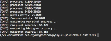

通过利用原始像素强度，我们能够达到54.42％的准确度。 另一方面，将k-NN应用于颜色直方图获得了略高的57.58％的准确度。可以看到，仅仅通过颜色直方图进行分类不是非常好的方法，对于具体案例来看，猫和狗的颜色可能是相同的，这样就存在误分类。当然这里是应用KNN做简单的分类实例，实际上非常容易的使用卷积神经网络能够达到95%以上的分类准确率。

下面讲一下利用knn算法进行分类

---

使用sklearn算法库进行参数调优，看看结果如何。

这里用到的是sklearn库中的grid search和random search函数对超参数组成的字典进行搜索，用knn算法模型度超参数字典搜索迭代。

代码：

# import the necessary packages
from sklearn.neighbors import KNeighborsClassifier
from sklearn.grid_search import RandomizedSearchCV
from sklearn.grid_search import GridSearchCV
from sklearn.cross_validation import train_test_split
from imutils import paths
import numpy as np
import argparse
import imutils
import time
import cv2
import os

def extract_color_histogram(image, bins=(8, 8, 8)):
	# extract a 3D color histogram from the HSV color space using
	# the supplied number of `bins` per channel
	hsv = cv2.cvtColor(image, cv2.COLOR_BGR2HSV)
	hist = cv2.calcHist([hsv], [0, 1, 2], None, bins,
		[0, 180, 0, 256, 0, 256])
 
	# handle normalizing the histogram if we are using OpenCV 2.4.X
	if imutils.is_cv2():
		hist = cv2.normalize(hist)
 
	# otherwise, perform "in place" normalization in OpenCV 3 (I
	# personally hate the way this is done
	else:
		cv2.normalize(hist, hist)
 
	# return the flattened histogram as the feature vector
	return hist.flatten()

# construct the argument parse and parse the arguments
ap = argparse.ArgumentParser()
ap.add_argument("-d", "--dataset", required=True,
	help="path to input dataset")
ap.add_argument("-j", "--jobs", type=int, default=-1,
	help="# of jobs for k-NN distance (-1 uses all available cores)")
args = vars(ap.parse_args())
 
# grab the list of images that we'll be describing
print("[INFO] describing images...")
imagePaths = list(paths.list_images(args["dataset"]))
 
# initialize the data matrix and labels list
data = []
labels = []

# loop over the input images
for (i, imagePath) in enumerate(imagePaths):
	# load the image and extract the class label (assuming that our
	# path as the format: /path/to/dataset/{class}.{image_num}.jpg
	image = cv2.imread(imagePath)
	label = imagePath.split(os.path.sep)[-1].split(".")[0]
 
	# extract a color histogram from the image, then update the
	# data matrix and labels list
	hist = extract_color_histogram(image)
	data.append(hist)
	labels.append(label)
 
	# show an update every 1,000 images
	if i > 0 and i % 1000 == 0:
		print("[INFO] processed {}/{}".format(i, len(imagePaths)))

# partition the data into training and testing splits, using 75%
# of the data for training and the remaining 25% for testing
print("[INFO] constructing training/testing split...")
(trainData, testData, trainLabels, testLabels) = train_test_split(
	data, labels, test_size=0.25, random_state=42)

# construct the set of hyperparameters to tune
params = {"n_neighbors": np.arange(1, 31, 2),
	"metric": ["euclidean", "cityblock"]}

# tune the hyperparameters via a cross-validated grid search
print("[INFO] tuning hyperparameters via grid search")
model = KNeighborsClassifier(n_jobs=args["jobs"])
grid = GridSearchCV(model, params)
start = time.time()
grid.fit(trainData, trainLabels)
 
# evaluate the best grid searched model on the testing data
print("[INFO] grid search took {:.2f} seconds".format(
	time.time() - start))
acc = grid.score(testData, testLabels)
print("[INFO] grid search accuracy: {:.2f}%".format(acc * 100))
print("[INFO] grid search best parameters: {}".format(
	grid.best_params_))

# tune the hyperparameters via a randomized search
grid = RandomizedSearchCV(model, params)
start = time.time()
grid.fit(trainData, trainLabels)
 
# evaluate the best randomized searched model on the testing
# data
print("[INFO] randomized search took {:.2f} seconds".format(
	time.time() - start))
acc = grid.score(testData, testLabels)
print("[INFO] grid search accuracy: {:.2f}%".format(acc * 100))
print("[INFO] randomized search best parameters: {}".format(
	grid.best_params_))

执行

python knn_tune.py --dataset kaggle_dogs_vs_cats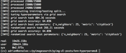

从输出屏幕截图中可以看出，网格搜索方法发现k = 25且metric ='cityblock'获得的最高准确度为64.03％。 但是，这次网格搜索耗时13分钟。另一方面，随机搜索获得了相同的64.03％的准确度 - 并且在5分钟内完成。所以在大多数情况下使用random search调优。