deep dream的体验和以往看论文,跑例子的过程完全不同。这是在跑“风格迁移”的例子时,在keras的examples中无意看到了程序,然后顺带跑一跑的。跑出来的效果让我觉得和无厘头,于是读程序,看它到底干了些啥。程序风格也很特别,没有和通常训练过程一般的迭代方式,又很好奇,处于什么目的做这个呢,于是,看了论文。看了论文,简直对写论文的人佩服的五体投地。整个过程笨妞的情绪就是一条“低开高走”的K线图。
所以,这篇文章的顺序是这样的:效果—>感受—>程序—>论文。
1. 效果
还是用那张今年春节在四川西昌邛海拍的“初春图”来做的。原图是这样的:
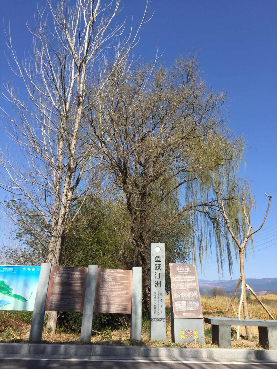
效果图是这样的:

2. 感受
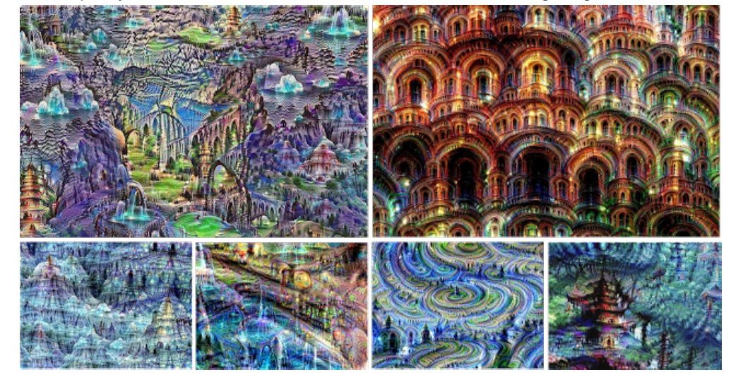
看到之后第一感觉是——imagenet里面是有多少"汪星人”的图片呀,搞得树上爬满了狗。这是做了“噩梦”吧。
于是上网搜了一下,据说要是拿人的照片来跑的话,“人变汪”的可能性比较大。好吧,幸好没拿自己的照片玩。
3. 程序
这个程序到底在干嘛!做了这么奇怪的梦。
程序是这样的:
'''Deep Dreaming in Keras.
Run the script with:
```
python deep_dream.py path_to_your_base_image.jpg prefix_for_results
```
e.g.:
```
python deep_dream.py img/mypic.jpg results/dream
```
'''
from __future__ import print_function


from keras.preprocessing.image import load_img, img_to_array
import numpy as np
import scipy
import argparse


from keras.applications import inception_v3
from keras import backend as K


parser = argparse.ArgumentParser(description='Deep Dreams with Keras.')
parser.add_argument('base_image_path', metavar='base', type=str,
                    help='Path to the image to transform.')
parser.add_argument('result_prefix', metavar='res', type=str,
                    help='Prefix for the saved results.')


args = parser.parse_args([ 'image/spring.jpg', 'deep_spring'])
base_image_path = args.base_image_path
result_prefix = args.result_prefix


# These are the names of the layers
# for which we try to maximize activation,
# as well as their weight in the final loss
# we try to maximize.
# You can tweak these setting to obtain new visual effects.


#定义要去抽取特征的模块,以及每个模块所占的权重
#在后面整合loss的时候用。
settings = {
    'features': {
        'mixed2': 0.2,
        'mixed3': 0.5,
        'mixed4': 2.,
        'mixed5': 1.5,
    },
}


#图像预处理。
#和“风格迁移”预处理过程一样,只是这里不是用vgg19的处理函数,用inception_v3的。
#因为我们的网络用inception v3
def preprocess_image(image_path):
    # Util function to open, resize and format pictures
    # into appropriate tensors.
    img = load_img(image_path)
    img = img_to_array(img)
    img = np.expand_dims(img, axis=0)
    img = inception_v3.preprocess_input(img)
    return img


#图像后处理,和“风格迁移”也差不多,把预处理是RGB->BRG的过程反过来。
def deprocess_image(x):
    # Util function to convert a tensor into a valid image.
    if K.image_data_format() == 'channels_first':
        x = x.reshape((3, x.shape[2], x.shape[3]))
        x = x.transpose((1, 2, 0))
    else:
        x = x.reshape((x.shape[1], x.shape[2], 3))
    x /= 2.
    x += 0.5
    x *= 255.
    x = np.clip(x, 0, 255).astype('uint8')
    return x


#将模式设置为训练
#0为训练,1为测试
K.set_learning_phase(0)


# Build the InceptionV3 network with our placeholder.
# The model will be loaded with pre-trained ImageNet weights.
#载入预训练模型
model = inception_v3.InceptionV3(weights='imagenet',
                                 include_top=False)
dream = model.input
print('Model loaded.')


# Get the symbolic outputs of each "key" layer (we gave them unique names).
#统计重要层
layer_dict = dict([(layer.name, layer) for layer in model.layers])


# Define the loss.
#定义loss
loss = K.variable(0.)
#抽出settings中各层的特征,并
for layer_name in settings['features']:
    # Add the L2 norm of the features of a layer to the loss.
    assert layer_name in layer_dict.keys(), 'Layer ' + layer_name + ' not found in model.'
    coeff = settings['features'][layer_name]
    x = layer_dict[layer_name].output
    # We avoid border artifacts by only involving non-border pixels in the loss.
    #scaling为所有特征图合起来的尺寸(x*y*channels)
    scaling = K.prod(K.cast(K.shape(x), 'float32'))
    #以像素值的平均平方值为该层的loss(为什么是这样的呢?)
    if K.image_data_format() == 'channels_first':
        loss += coeff * K.sum(K.square(x[:, :, 2: -2, 2: -2])) / scaling
    else:
        loss += coeff * K.sum(K.square(x[:, 2: -2, 2: -2, :])) / scaling


# Compute the gradients of the dream wrt the loss.
#计算loss基于dream(模型输入)的梯度
grads = K.gradients(loss, dream)[0]
# Normalize gradients.
#梯度归一化
grads /= K.maximum(K.mean(K.abs(grads)), K.epsilon())


# Set up function to retrieve the value
# of the loss and gradients given an input image.
#定义迭代计算图
outputs = [loss, grads]
fetch_loss_and_grads = K.function([dream], outputs)


#获取loss和梯度
def eval_loss_and_grads(x):
    outs = fetch_loss_and_grads([x])
    loss_value = outs[0]
    grad_values = outs[1]
    return loss_value, grad_values


def resize_img(img, size):
    img = np.copy(img)
    if K.image_data_format() == 'channels_first':
        factors = (1, 1,
                   float(size[0]) / img.shape[2],
                   float(size[1]) / img.shape[3])
    else:
        factors = (1,
                   float(size[0]) / img.shape[1],
                   float(size[1]) / img.shape[2],
                   1)
    #order=1按照双线性变换的方法插值。
    return scipy.ndimage.zoom(img, factors, order=1)


#优化过程,按照step和迭代次数,逐次优化,优化方式是将梯度值叠加到x上。
def gradient_ascent(x, iterations, step, max_loss=None):
    for i in range(iterations):
        loss_value, grad_values = eval_loss_and_grads(x)
        if max_loss is not None and loss_value > max_loss:
            break
        print('..Loss value at', i, ':', loss_value)
        x += step * grad_values
    return x


def save_img(img, fname):
    pil_img = deprocess_image(np.copy(img))
    scipy.misc.imsave(fname, pil_img)


"""Process:
- Load the original image.
- Define a number of processing scales (i.e. image shapes),
    from smallest to largest.
- Resize the original image to the smallest scale.
- For every scale, starting with the smallest (i.e. current one):
    - Run gradient ascent
    - Upscale image to the next scale
    - Reinject the detail that was lost at upscaling time
- Stop when we are back to the original size.
To obtain the detail lost during upscaling, we simply
take the original image, shrink it down, upscale it,
and compare the result to the (resized) original image.
"""


#迭代正式开始......


# Playing with these hyperparameters will also allow you to achieve new effects
step = 0.01  # Gradient ascent step size
num_octave = 3  # Number of scales at which to run gradient ascent
octave_scale = 1.4  # Size ratio between scales
iterations = 20  # Number of ascent steps per scale
max_loss = 10.


#原始图像预处理
img = preprocess_image(base_image_path)
if K.image_data_format() == 'channels_first':
    original_shape = img.shape[2:]
else:
    original_shape = img.shape[1:3]
#定义图像shape的变化层次
#随着迭代,successive_shape越来越小,这是什么原理呢?图像金字塔,多尺寸?
successive_shapes = [original_shape]
for i in range(1, num_octave):
    #根据octave_scale同比例缩小图像
    shape = tuple([int(dim / (octave_scale ** i)) for dim in original_shape])
    successive_shapes.append(shape)
print(successive_shapes)
#顺序方向,图像从小往大处理,那么处理到最后,和原图像一样大。
successive_shapes = successive_shapes[::-1]
original_img = np.copy(img)
#在迭代开始前首先将图像resize小。
shrunk_original_img = resize_img(img, successive_shapes[0])


#这个迭代和平时见到的迭代不同,平时是所有数据所有情况跑一边算一次迭代。
#这里,一个shape跑完所有迭代次数,然后进入下一个shape.
#shape的意义还是不清楚。
for shape in successive_shapes:
    print('Processing image shape', shape)
    #根据预定义的shape变化层次resize图像
    img = resize_img(img, shape)
    #优化图像
    img = gradient_ascent(img,
                          iterations=iterations,
                          step=step,
                          max_loss=max_loss)
    upscaled_shrunk_original_img = resize_img(shrunk_original_img, shape)
    same_size_original = resize_img(original_img, shape)
    #原始图经过当前shape zoom与经过前一次和当前次shape两次zoom的差值为lost_detail
    lost_detail = same_size_original - upscaled_shrunk_original_img

    #每次迭代生成图像由输入图像(上一次迭代的输出)+ 逐次迭代的梯度和 + 基本损失折算到每个shape下的损失 组合而成
    img += lost_detail
    shrunk_original_img = resize_img(original_img, shape)


    #保存图像
save_img(img, fname=result_prefix + '.png')
从程序上来看,这就是跑一遍inception v3网络,然后,从网络第2、3、4、5块抽出输出特征图,然后以每块的像素值的平方平均值作为loss,对dream图求梯度,用这个梯度来优化dream图。迭代以iterations和successive_shapes两个维度控制,前者控制梯度优化的次数,后者控制dream图的shape变化。程序实例中,图像是渐进式处理的,先将图像缩小,然后再逐次放大,每放大一次,跑一次全iterations的全迭代过程。图像由小往大迭代的意义是否和多尺度处理相同呢?这点暂时有点困惑。
4. 论文翻译
在读论文时,发现整个论文都比较有意义,所以整篇翻译了来。论文只写了基本思想,实现方法一笔带过。
####################################论文翻译在此########################################


#########################################论文结束###################################
至此,终于明白这个idea的发明者要做什么了。简直太有想法了有木有!
回想一下自己的梦境,经常就是很无厘头,说不清道不明,说不定我们的梦境就是大脑皮层某些神经元抽取白天的场景的一些特征,融合融合形成的呢。
而且通过以有监督的学习为手段,以提取特征为目的,抽取特征,也是替代人工劳力很棒的方式呀。