Spark MLlib之分类模型源码分析

权重更新

MLlib采用如下方式更新模型（LR、SVM、线性回归等）的权重：

w' = w - t h i s I t e r S t e p S i z e * (g r a d i e n t + r e g P a r a m * w)

$w' = w - thisIterStepSize * (gradient + regParam * w)$

w' = (1 - t h i s I t e r S t e p S i z e * r e g P a r a m) * w - t h i s I t e r S t e p S i z e * g r a d i e n t

$w' = (1 - thisIterStepSize * regParam) * w - thisIterStepSize * gradient$

逻辑回归（LR）回顾

Logistic regression是机器学习常用的分类模型，用于将不同样本分开。本文的重点不在Logistic regression的细节，关于Logistic regression的具体原理和公式推导请参考zuoxy09的博文—— 机器学习算法与Python实践之（七）逻辑回归（Logistic Regression）。
接下来给出Logistic regression的cost function：

J (θ) = - [1 m \sum i = 1 m y (i) log h θ (x (i)) + (1 - y (i)) log (1 - h θ (x (i)))] + λ 2 m \sum j = 1 n θ 2 j

$J(\theta) =- \left[\frac1m\sum_{i=1}^my^{(i)}\log^{h_\theta(x^{(i)})} + (1-y^{(i)})\log^{(1-h_\theta(x^{(i)}))}\right] +\frac\lambda{2m}\sum_{j=1}^n\theta_j^2$
使用梯度下降（Gradient Descent），对

J(θ) $J(θ)$ 求导等于0，得到

θj $θ_j$

θ j + 1 = θ j - α [1 m \sum i = 1 m (h θ (x (i)) - y (i)) x (i) j + λ m θ j]

$\theta_{j+1} = \theta_j - \alpha\left[\frac1m\sum_{i=1}^m(h_\theta(x^{(i)})-y^{(i)})x_j^{(i)} + \frac\lambda{m}\theta_j\right]$
对于梯度下降的方法，请参考—— 随机梯度下降与批量梯度下降。
对上面的式子做如下变换：

θ j + 1 = θ j (1 - α λ m) - α 1 m \sum i = 1 m (h θ (x (i)) - y (i)) x (i) j

$\theta_{j+1} = \theta_j(1-\alpha\frac\lambda{m}) -\alpha\frac1m\sum_{i=1}^m(h_\theta(x^{(i)})-y^{(i)})x_j^{(i)}$

并行的梯度下降

梯度下降MapReduce实现
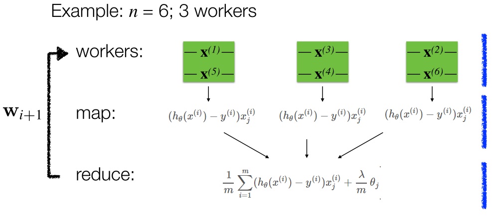
其中：
map函数计算每个点的梯度： $(h_\theta(x^{(i)})-y^{(i)})x_j^{(i)}$ ；
reduce函数计算所有点的梯度求和以及正则项： $\frac1m\sum_{i=1}^m(h_\theta(x^{(i)})-y^{(i)})x_j^{(i)} + \frac\lambda{m}\theta_j$ ；

Mlib源码分析

Logistic regression利用梯度下降求解参数 $\theta_j$ 核心代码在GradientDescent#runMiniBatchSGD方法中，包括两部分

/**
  * 
  * @param data 样本数据RDD，格式 (label, [features])
  * @param gradient 对应LogisticGradient，用于计算每个样本梯度及误差
  * @param updater 对应SquaredL2Updater, 用于每次更新权重
  * @param stepSize 初始步长
  * @param numIterations 迭代次数
  * @param regParam 正则化因子
  * @param miniBatchFraction 每次迭代参与计算的样本比例
  * @param convergenceTol 迭代前后的变化，小于某个阈值停止迭代
  * @return (Vector, Array[Double]) 第一个为权重，每二个为每次迭代的误差值
*/
def runMiniBatchSGD(
    data: RDD[(Double, Vector)],
    gradient: Gradient,
    updater: Updater,
    stepSize: Double,
    numIterations: Int,
    regParam: Double,
    miniBatchFraction: Double,
    initialWeights: Vector,
    convergenceTol: Double): (Vector, Array[Double]) = {

  // 误差变化历史记录
  val stochasticLossHistory = new ArrayBuffer[Double](numIterations)
  // Record previous weight and current one to calculate solution vector difference
  var previousWeights: Option[Vector] = None
  var currentWeights: Option[Vector] = None
  val numExamples = data.count()
  // Initialize weights as a column vector
  var weights = Vectors.dense(initialWeights.toArray)
  val n = weights.size
  // 第一次迭代初始化正则因子
  var regVal = updater.compute(
    weights, Vectors.zeros(weights.size), 0, 1, regParam)._2
  // indicates whether converged based on convergenceTol
  var converged = false 
  var i = 1
  while (!converged && i <= numIterations) {
    val bcWeights = data.context.broadcast(weights)
    // Sample a subset (fraction miniBatchFraction) of the total data
    // compute and sum up the subgradients on this subset (this is one map-reduce)
    // treeAggregate的使用请参考http://stackoverflow.com/questions/29860635/how-to-interpret-rdd-treeaggregate
    // 计算梯度和误差
    val (gradientSum, lossSum, miniBatchSize) = data.sample(false, miniBatchFraction, 42 + i)
      .treeAggregate((BDV.zeros[Double](n), 0.0, 0L))(
        seqOp = (c, v) => {
          // c: (grad, loss, count), v: (label, features)
          val loss = gradient.compute(v._2, v._1, bcWeights.value, Vectors.fromBreeze(c._1))
          (c._1, c._2 + loss, c._3 + 1)
        },
        combOp = (c1, c2) => {
          // c: (grad, loss, count)
          (c1._1 += c2._1, c1._2 + c2._2, c1._3 + c2._3)
        })

    if (miniBatchSize > 0) {
      stochasticLossHistory.append(lossSum / miniBatchSize + regVal)
      // 更新梯度
      val update = updater.compute(
        weights, Vectors.fromBreeze(gradientSum / miniBatchSize.toDouble),
        stepSize, i, regParam)
      weights = update._1
      regVal = update._2

      previousWeights = currentWeights
      currentWeights = Some(weights)
      if (previousWeights != None && currentWeights != None) {
        converged = isConverged(previousWeights.get,
          currentWeights.get, convergenceTol)
      }
    } else {
      logWarning(s"Iteration ($i/$numIterations). The size of sampled batch is zero")
    }
    i += 1
  }
  (weights, stochasticLossHistory.toArray)
}

上面方法中包含两部分：
1、计算梯度gradient.compute

\sum i = 1 m (h θ (x (i)) - y (i)) x (i) j

$\sum_{i=1}^m(h_\theta(x^{(i)})-y^{(i)})x_j^{(i)}$

override def compute(
      data: Vector,
      label: Double,
      weights: Vector,
      cumGradient: Vector): Double = {
    val dataSize = data.size
    val margin = -1.0 * dot(data, weights)
    // 公式（2）中求和部分
    val multiplier = (1.0 / (1.0 + math.exp(margin))) - label
    // cumGradient为当前累计求和后的梯度
    // cumGradient += multiplier * data
    axpy(multiplier, data, cumGradient)
    // 误差
    if (label > 0) {
      // The following is equivalent to log(1 + exp(margin)) but more numerically stable.
      MLUtils.log1pExp(margin)
    } else {
      MLUtils.log1pExp(margin) - margin
    }
}

2、更新权重updater.compute

θ j + 1 = θ j (1 - α λ m) - α * g r a d i e n t

$\theta_{j+1} = \theta_j(1-\alpha\frac\lambda{m}) -\alpha * gradient$

override def compute(
      weightsOld: Vector,
      gradient: Vector,
      stepSize: Double,
      iter: Int,
      regParam: Double): (Vector, Double) = {
    // 本次迭代步长alpha
    val thisIterStepSize = stepSize / math.sqrt(iter)
    // 根据公式（3）计算权重，brzWeights为当前权重theta
    val brzWeights: BV[Double] = weightsOld.toBreeze.toDenseVector
    // :* 为向量scalar计算
    brzWeights :*= (1.0 - thisIterStepSize * regParam)
    // brzWeights += -thisIterStepSize * gradient
    brzAxpy(-thisIterStepSize, gradient.toBreeze, brzWeights)
    // 正则项
    val norm = brzNorm(brzWeights, 2.0)
    (Vectors.fromBreeze(brzWeights), 0.5 * regParam * norm * norm)
  }

线性SVM

cost function：

J (θ) = 1 m \sum i = 1 m m a x (0, 1 - y (i) h θ (x (i))) + λ 2 m \sum j = 1 n θ 2 j

$J(\theta) = \frac1m\sum_{i=1}^m max(0, 1 - y^{(i)}h_\theta(x^{(i)}) )+ \frac\lambda{2m}\sum_{j=1}^n\theta_j^2$
注：

hθ(x(i))=θTx(i) $h_\theta(x^{(i)}) =\theta^Tx^{(i)}$
使用梯度下降（Gradient Descent），对

J(θ) $J(θ)$ 求导等于0，得到

θ $θ$

θ j + 1 = {θ j - α (λ θ j - 1 m \sum m i = 1 y (i) x (i)), θ j - α λ θ j, if y (i) h θ (x (i)) < 1 otherwise

$\theta_{j+1} = \begin{cases} \theta_j - \alpha(\lambda\theta_j -\frac1m\sum_{i=1}^m y^{(i)}x^{(i)}),& \text{if } y^{(i)}h_\theta(x^{(i)}) < 1\\ \theta_j - \alpha\lambda\theta_j, & \text{otherwise} \end{cases}$
关于SVM参数计算推导见这里。

−y(i)x(i) $−y^{(i)}x^{(i)}$ 为梯度。