分类与回归

一、分类

1. 逻辑分类

Logistic回归是一种用于预测分类响应的流行方法。这是广义线性模型的一种特殊情况，可以预测结果的可能性。在spark.ml中，逻辑回归可以通过使用二项式逻辑回归来预测二进制结果，或者可以通过使用多项逻辑回归来预测多类结果。使用family参数在这两种算法之间进行选择，或者不设置它，Spark会推断出正确的变体。
通过将family参数设置为“multinomial”，可以将多项式逻辑回归用于二进制分类。它将产生两组系数和两个截距。
当对具有恒定非零列的数据集进行LogisticRegressionModel拟合而没有截距时，Spark MLlib为恒定非零列输出零系数。此行为与R glmnet相同，但与LIBSVM不同。

1.1 二元逻辑回归

有关二项式逻辑回归的实现的更多背景和更多详细信息，请参阅spark.mllib中的逻辑回归文档。

from pyspark.ml.classification import LogisticRegression

# Load training data
training = spark.read.format("libsvm").load("data/mllib/sample_libsvm_data.txt")

lr = LogisticRegression(maxIter=10, regParam=0.3, elasticNetParam=0.8)

# Fit the model
lrModel = lr.fit(training)

# Print the coefficients and intercept for logistic regression
print("Coefficients: " + str(lrModel.coefficients))
print("Intercept: " + str(lrModel.intercept))

# We can also use the multinomial family for binary classification
mlr = LogisticRegression(maxIter=10, regParam=0.3, elasticNetParam=0.8, family="multinomial")

# Fit the model
mlrModel = mlr.fit(training)

# Print the coefficients and intercepts for logistic regression with multinomial family
print("Multinomial coefficients: " + str(mlrModel.coefficientMatrix))
print("Multinomial intercepts: " + str(mlrModel.interceptVector))

LogisticRegressionTrainingSummary提供LogisticRdgressionModel的总结。在二进制分类的情况下，某些其他指标可用，例如ROC曲线。可以通过binarySummary方法访问binary summary

from pyspark.ml.classification import LogisticRegression

# Extract the summary from the returned LogisticRegressionModel instance trained
# in the earlier example
trainingSummary = lrModel.summary

# Obtain the objective per iteration
objectiveHistory = trainingSummary.objectiveHistory
print("objectiveHistory:")
for objective in objectiveHistory:
    print(objective)

# Obtain the receiver-operating characteristic as a dataframe and areaUnderROC.
trainingSummary.roc.show()
print("areaUnderROC: " + str(trainingSummary.areaUnderROC))

# Set the model threshold to maximize F-Measure
fMeasure = trainingSummary.fMeasureByThreshold
maxFMeasure = fMeasure.groupBy().max('F-Measure').select('max(F-Measure)').head()
bestThreshold = fMeasure.where(fMeasure['F-Measure'] == maxFMeasure['max(F-Measure)']) \
    .select('threshold').head()['threshold']
lr.setThreshold(bestThreshold)

1.2 多项逻辑回归

通过多项逻辑（softmax）回归支持多类别分类。在多项逻辑回归中，该算法会生成K个系数集，或一个尺寸为K×J的矩阵，其中K是结果类的数量，J是特征的数量。
多项式系数可作为cofficientMatirx使用，截距可作为interceptVector使用

from pyspark.ml.classification import LogisticRegression

# Load training data
training = spark \
    .read \
    .format("libsvm") \
    .load("data/mllib/sample_multiclass_classification_data.txt")

lr = LogisticRegression(maxIter=10, regParam=0.3, elasticNetParam=0.8)

# Fit the model
lrModel = lr.fit(training)

# Print the coefficients and intercept for multinomial logistic regression
print("Coefficients: \n" + str(lrModel.coefficientMatrix))
print("Intercept: " + str(lrModel.interceptVector))

trainingSummary = lrModel.summary

# Obtain the objective per iteration
objectiveHistory = trainingSummary.objectiveHistory
print("objectiveHistory:")
for objective in objectiveHistory:
    print(objective)

# for multiclass, we can inspect metrics on a per-label basis
print("False positive rate by label:")
for i, rate in enumerate(trainingSummary.falsePositiveRateByLabel):
    print("label %d: %s" % (i, rate))

print("True positive rate by label:")
for i, rate in enumerate(trainingSummary.truePositiveRateByLabel):
    print("label %d: %s" % (i, rate))

print("Precision by label:")
for i, prec in enumerate(trainingSummary.precisionByLabel):
    print("label %d: %s" % (i, prec))

print("Recall by label:")
for i, rec in enumerate(trainingSummary.recallByLabel):
    print("label %d: %s" % (i, rec))

print("F-measure by label:")
for i, f in enumerate(trainingSummary.fMeasureByLabel()):
    print("label %d: %s" % (i, f))

accuracy = trainingSummary.accuracy
falsePositiveRate = trainingSummary.weightedFalsePositiveRate
truePositiveRate = trainingSummary.weightedTruePositiveRate
fMeasure = trainingSummary.weightedFMeasure()
precision = trainingSummary.weightedPrecision
recall = trainingSummary.weightedRecall
print("Accuracy: %s\nFPR: %s\nTPR: %s\nF-measure: %s\nPrecision: %s\nRecall: %s"
      % (accuracy, falsePositiveRate, truePositiveRate, fMeasure, precision, recall))

2 决策树

以下示例以LibSVM格式加载数据集，将其分为训练集和测试集，在第一个数据集上进行训练，然后对保留的测试集进行评估。我们使用两个特征转换器准备数据。这些帮助为标签和分类功能的索引类别，将元数据添加到决策树算法可以识别的DataFrame中。

from pyspark.ml import Pipeline
from pyspark.ml.classification import DecisionTreeClassifier
from pyspark.ml.feature import StringIndexer, VectorIndexer
from pyspark.ml.evaluation import MulticlassClassificationEvaluator

# Load the data stored in LIBSVM format as a DataFrame.
data = spark.read.format("libsvm").load("data/mllib/sample_libsvm_data.txt")

# Index labels, adding metadata to the label column.
# Fit on whole dataset to include all labels in index.
labelIndexer = StringIndexer(inputCol="label", outputCol="indexedLabel").fit(data)
# Automatically identify categorical features, and index them.
# We specify maxCategories so features with > 4 distinct values are treated as continuous.
featureIndexer =\
    VectorIndexer(inputCol="features", outputCol="indexedFeatures", maxCategories=4).fit(data)

# Split the data into training and test sets (30% held out for testing)
(trainingData, testData) = data.randomSplit([0.7, 0.3])

# Train a DecisionTree model.
dt = DecisionTreeClassifier(labelCol="indexedLabel", featuresCol="indexedFeatures")

# Chain indexers and tree in a Pipeline
pipeline = Pipeline(stages=[labelIndexer, featureIndexer, dt])

# Train model.  This also runs the indexers.
model = pipeline.fit(trainingData)

# Make predictions.
predictions = model.transform(testData)

# Select example rows to display.
predictions.select("prediction", "indexedLabel", "features").show(5)

# Select (prediction, true label) and compute test error
evaluator = MulticlassClassificationEvaluator(
    labelCol="indexedLabel", predictionCol="prediction", metricName="accuracy")
accuracy = evaluator.evaluate(predictions)
print("Test Error = %g " % (1.0 - accuracy))

treeModel = model.stages[2]
# summary only
print(treeModel)

3.随机森林分类

以下示例以LibSVM格式加载数据集，将其分为训练集和测试集，在第一个数据集上进行训练，然后对保留的测试集进行评估。我们使用两个特征转换器准备数据。这些帮助为标签和分类功能的索引类别，将元数据添加到基于树的算法可以识别的DataFrame中。

from pyspark.ml import Pipeline
from pyspark.ml.classification import RandomForestClassifier
from pyspark.ml.feature import IndexToString, StringIndexer, VectorIndexer
from pyspark.ml.evaluation import MulticlassClassificationEvaluator

# Load and parse the data file, converting it to a DataFrame.
data = spark.read.format("libsvm").load("data/mllib/sample_libsvm_data.txt")

# Index labels, adding metadata to the label column.
# Fit on whole dataset to include all labels in index.
labelIndexer = StringIndexer(inputCol="label", outputCol="indexedLabel").fit(data)

# Automatically identify categorical features, and index them.
# Set maxCategories so features with > 4 distinct values are treated as continuous.
featureIndexer =\
    VectorIndexer(inputCol="features", outputCol="indexedFeatures", maxCategories=4).fit(data)

# Split the data into training and test sets (30% held out for testing)
(trainingData, testData) = data.randomSplit([0.7, 0.3])

# Train a RandomForest model.
rf = RandomForestClassifier(labelCol="indexedLabel", featuresCol="indexedFeatures", numTrees=10)

# Convert indexed labels back to original labels.
labelConverter = IndexToString(inputCol="prediction", outputCol="predictedLabel",
                               labels=labelIndexer.labels)

# Chain indexers and forest in a Pipeline
pipeline = Pipeline(stages=[labelIndexer, featureIndexer, rf, labelConverter])

# Train model.  This also runs the indexers.
model = pipeline.fit(trainingData)

# Make predictions.
predictions = model.transform(testData)

# Select example rows to display.
predictions.select("predictedLabel", "label", "features").show(5)

# Select (prediction, true label) and compute test error
evaluator = MulticlassClassificationEvaluator(
    labelCol="indexedLabel", predictionCol="prediction", metricName="accuracy")
accuracy = evaluator.evaluate(predictions)
print("Test Error = %g" % (1.0 - accuracy))

rfModel = model.stages[2]
print(rfModel)  # summary only

4. 梯度提升树

from pyspark.ml import Pipeline
from pyspark.ml.classification import GBTClassifier
from pyspark.ml.feature import StringIndexer, VectorIndexer
from pyspark.ml.evaluation import MulticlassClassificationEvaluator

# Load and parse the data file, converting it to a DataFrame.
data = spark.read.format("libsvm").load("data/mllib/sample_libsvm_data.txt")

# Index labels, adding metadata to the label column.
# Fit on whole dataset to include all labels in index.
labelIndexer = StringIndexer(inputCol="label", outputCol="indexedLabel").fit(data)
# Automatically identify categorical features, and index them.
# Set maxCategories so features with > 4 distinct values are treated as continuous.
featureIndexer =\
    VectorIndexer(inputCol="features", outputCol="indexedFeatures", maxCategories=4).fit(data)

# Split the data into training and test sets (30% held out for testing)
(trainingData, testData) = data.randomSplit([0.7, 0.3])

# Train a GBT model.
gbt = GBTClassifier(labelCol="indexedLabel", featuresCol="indexedFeatures", maxIter=10)

# Chain indexers and GBT in a Pipeline
pipeline = Pipeline(stages=[labelIndexer, featureIndexer, gbt])

# Train model.  This also runs the indexers.
model = pipeline.fit(trainingData)

# Make predictions.
predictions = model.transform(testData)

# Select example rows to display.
predictions.select("prediction", "indexedLabel", "features").show(5)

# Select (prediction, true label) and compute test error
evaluator = MulticlassClassificationEvaluator(
    labelCol="indexedLabel", predictionCol="prediction", metricName="accuracy")
accuracy = evaluator.evaluate(predictions)
print("Test Error = %g" % (1.0 - accuracy))

gbtModel = model.stages[2]
print(gbtModel)  # summary only

5. 多层感知器

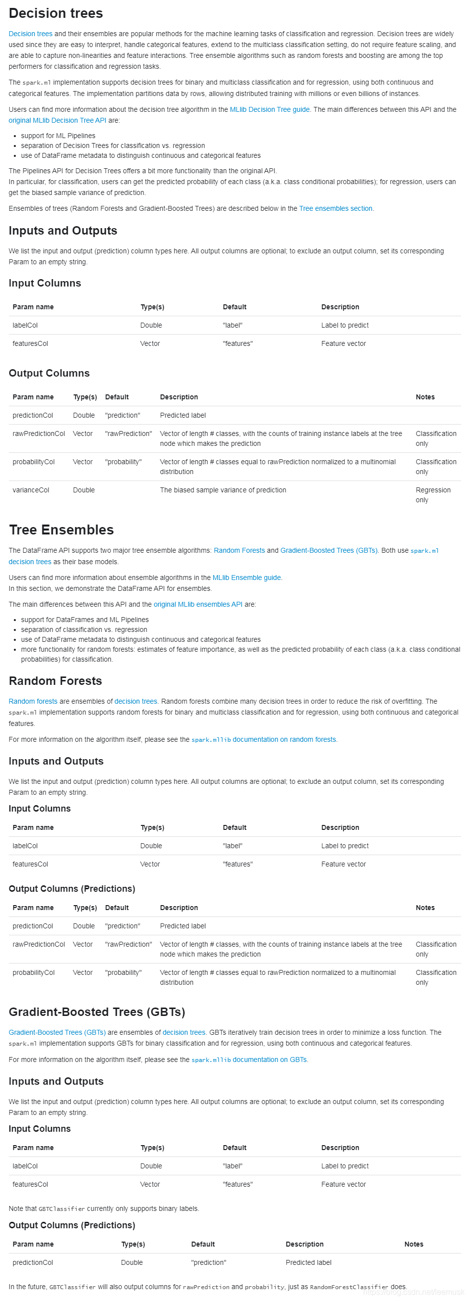
多层感知器分类器（MLPC）是基于前馈人工神经网络的分类器。 MLPC由多层节点组成。每一层都完全连接到网络中的下一层。输入层中的节点代表输入数据。所有其他节点通过输入与节点权重w和偏差b的线性组合并应用激活函数，将输入映射到输出。对于具有K + 1层的MLPC，可以将其写成矩阵形式，如下所示：
在这里插入图片描述
中间层中的节点使用激活函数

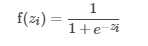
输出层中的节点使用softmax函数：

输出层中节点N的数量与类的数量相对应。 MLPC使用反向传播来学习模型。我们使用逻辑损失函数进行优化，并使用L-BFGS作为优化例程。

from pyspark.ml.classification import MultilayerPerceptronClassifier
from pyspark.ml.evaluation import MulticlassClassificationEvaluator

# Load training data
data = spark.read.format("libsvm")\
    .load("data/mllib/sample_multiclass_classification_data.txt")

# Split the data into train and test
splits = data.randomSplit([0.6, 0.4], 1234)
train = splits[0]
test = splits[1]

# specify layers for the neural network:
# input layer of size 4 (features), two intermediate of size 5 and 4
# and output of size 3 (classes)
layers = [4, 5, 4, 3]

# create the trainer and set its parameters
trainer = MultilayerPerceptronClassifier(maxIter=100, layers=layers, blockSize=128, seed=1234)

# train the model
model = trainer.fit(train)

# compute accuracy on the test set
result = model.transform(test)
predictionAndLabels = result.select("prediction", "label")
evaluator = MulticlassClassificationEvaluator(metricName="accuracy")
print("Test set accuracy = " + str(evaluator.evaluate(predictionAndLabels)))

6. 线性支持向量机

支持向量机在高维或无限维空间中构造一个超平面或一组超平面，可用于分类，回归或其他任务。直观地，通过超平面可以实现良好的分离，该超平面与任何类别的最近训练数据点之间的距离最大（所谓的功能裕度），因为通常裕度越大，分类器的泛化误差越低。 Spark ML中的LinearSVC支持使用线性SVM进行二进制分类。在内部，它使用OWLQN优化器优化Hinge Loss
Hinge Loss：用于训练分类器的损失函数，常被用于最大间隔分类。定义：
$l(y) = max(0, 1 - t \cdot y)$
t为预期输出+1， -1；y为分类器的"原始输出"。当 t 和 y 符号相同(即 y 分类正确)，且 $|y|\geq 1$ 时，铰接损失 $\ell (y)=0$ 。但当它们符号相反， $\ell (y)$ 随 y 线性增长（分类错误）。类似的，如果 $|y|<1$ ，即使 t 和 y 符号相同(正确分类，但分类间隔不足) 也会有损失。

from pyspark.ml.classification import LinearSVC

# Load training data
training = spark.read.format("libsvm").load("data/mllib/sample_libsvm_data.txt")

lsvc = LinearSVC(maxIter=10, regParam=0.1)

# Fit the model
lsvcModel = lsvc.fit(training)

# Print the coefficients and intercept for linear SVC
print("Coefficients: " + str(lsvcModel.coefficients))
print("Intercept: " + str(lsvcModel.intercept))

7. one-vs-rest / one-vs-all

OneVsRest是机器学习简化的一个示例，它提供了可以有效执行二进制分类的基本分类器，从而可以执行多分类。它也被称为“一对多”。OneVsRest被实现为一个估计器。对于基本分类器，它采用分类器的实例，并为k个类的每一个创建一个二进制分类问题。训练类别i的分类器以预测标签是否为i，从而将类别i与所有其他类别区分开。预测是通过评估每个二进制分类器来完成的，最可靠的分类器的索引将作为标签输出。

from pyspark.ml.classification import LogisticRegression, OneVsRest
from pyspark.ml.evaluation import MulticlassClassificationEvaluator

# load data file.
inputData = spark.read.format("libsvm") \
    .load("data/mllib/sample_multiclass_classification_data.txt")

# generate the train/test split.
(train, test) = inputData.randomSplit([0.8, 0.2])

# instantiate the base classifier.
lr = LogisticRegression(maxIter=10, tol=1E-6, fitIntercept=True)

# instantiate the One Vs Rest Classifier.
ovr = OneVsRest(classifier=lr)

# train the multiclass model.
ovrModel = ovr.fit(train)

# score the model on test data.
predictions = ovrModel.transform(test)

# obtain evaluator.
evaluator = MulticlassClassificationEvaluator(metricName="accuracy")

# compute the classification error on test data.
accuracy = evaluator.evaluate(predictions)
print("Test Error = %g" % (1.0 - accuracy))

8.朴素贝叶斯

朴素贝叶斯分类器是一系列简单的概率分类器，基于贝叶斯定理，在每对特征之间使用强（朴素）独立性假设。朴素贝叶斯可以非常有效地训练。通过一次传递训练数据，就可以计算给定每个标签的每个特征的条件概率分布。为了进行预测，它使用贝叶斯定理来计算给定观察结果的每个标签的条件概率分布。 MLlib支持多项式朴素贝叶斯和Bernoulli朴素贝叶斯。输入数据：这些模型通常用于文档分类。在这种情况下，每个观察结果都是一个文档，每个功能都代表一个术语。特征值是术语的频率（在多项式朴素贝叶斯中），或者为零或一，表示是否在文档中找到了该术语（在Bernoulli Naive Bayes中）。特征值必须为非负数。使用可选参数“ multinomial”或“ bernoulli”（默认值为“ multinomial”）选择模型类型。对于文档分类，输入特征向量通常应为稀疏向量。由于训练数据仅使用一次，因此无需将其缓存。可以通过设置参数λ（默认值为1.0）来使用加法平滑。

from pyspark.ml.classification import NaiveBayes
from pyspark.ml.evaluation import MulticlassClassificationEvaluator

# Load training data
data = spark.read.format("libsvm") \
    .load("data/mllib/sample_libsvm_data.txt")

# Split the data into train and test
splits = data.randomSplit([0.6, 0.4], 1234)
train = splits[0]
test = splits[1]

# create the trainer and set its parameters
nb = NaiveBayes(smoothing=1.0, modelType="multinomial")

# train the model
model = nb.fit(train)

# select example rows to display.
predictions = model.transform(test)
predictions.show()

# compute accuracy on the test set
evaluator = MulticlassClassificationEvaluator(labelCol="label", predictionCol="prediction",
                                              metricName="accuracy")
accuracy = evaluator.evaluate(predictions)
print("Test set accuracy = " + str(accuracy))

二、回归

1. 线性分类

用于线性回归模型和模型摘要的接口类似于逻辑回归情况。
当通过“ l-bfgs”求解器拟合

当通过“ l-bfgs”求解器拟合具有恒定非零列的数据集而没有截距的LinearRegressionModel时，Spark MLlib为恒定非零列输出零系数。此行为与R glmnet相同，但与LIBSVM不同。

from pyspark.ml.regression import LinearRegression

# Load training data
training = spark.read.format("libsvm")\
    .load("data/mllib/sample_linear_regression_data.txt")

lr = LinearRegression(maxIter=10, regParam=0.3, elasticNetParam=0.8)

# Fit the model
lrModel = lr.fit(training)

# Print the coefficients and intercept for linear regression
print("Coefficients: %s" % str(lrModel.coefficients))
print("Intercept: %s" % str(lrModel.intercept))

# Summarize the model over the training set and print out some metrics
trainingSummary = lrModel.summary
print("numIterations: %d" % trainingSummary.totalIterations)
print("objectiveHistory: %s" % str(trainingSummary.objectiveHistory))
trainingSummary.residuals.show()
print("RMSE: %f" % trainingSummary.rootMeanSquaredError)
print("r2: %f" % trainingSummary.r2)

2. 广义线性回归

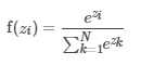
与线性回归（假设输出遵循高斯分布）相反，广义线性模型（GLM）是线性模型的规范，其中响应变量Yi遵循指数分布族的某种分布。 Spark的GeneralizedLinearRegression接口可以灵活地指定GLM，可用于各种类型的预测问题，包括线性回归，泊松回归，逻辑回归等。当前在spark.ml中，仅支持指数族分布的子集，并在下面列出。
Spark目前仅通过其GeneralizedLinearRegression接口最多支持4096个特征，如果超出此约束，将引发异常。
GLM需要指数族分布，可以以其“规范”或“自然”形式（也称为自然指数族分布）来编写。自然指数族分布的形式为：
$f_Y(y|θ,τ)=h(y,τ)exp(\frac{θ⋅y−A(θ)}{d(τ)})$

其中θ是parameter of interest，而τ是dispersion parameter。在GLM中，假定响应变量Yi从自然指数族分布中得出:
在这里插入图片描述
其中parameter of interestθi与期望值相关响应变量μi的值由 $μi= A'（θi）$ 在这里， $A'（θi）$ 由所选分布的形式定义。 GLM还允许指定链接函数，该链接函数定义了响应变量 $μi$ 的期望值与所谓的线性预测变量 $ηi$ 之间的关系：
$g(\mu_i) = \eta_i = \vec{x_i}^T \cdot \vec{\beta}$
通常，选择链接函数以使 $A'= g-1$ ，这在感兴趣的参数θ和线性预测变量η之间产生简化的关系。在这种情况下，链接函数 $g（μ）$ 被称为“规范”链接函数。
$\theta_i = A'^{-1}(\mu_i) = g(g^{-1}(\eta_i)) = \eta_i$
A GLM找到回归系数 $\vec{\beta}$ 最大化似然函数。 $\max_{\vec{\beta}} \mathcal{L}(\vec{\theta}|\vec{y},X) = \prod_{i=1}^{N} h(y_i, \tau) \exp{\left(\frac{y_i\theta_i - A(\theta_i)}{d(\tau)}\right)}$ ，其中 parameter of interest $θi$ 与回归系数 $\vec{\beta}$ 通过
$\theta_i = A'^{-1}(g^{-1}(\vec{x_i} \cdot \vec{\beta}))$ Spark的广义线性回归接口还提供了用于诊断GLM模型拟合的摘要统计信息，包括残差，p值，偏差，Akaike信息准则，和其他的。

Family	Response Type	Supported Links
Gaussian	Continuous	Identity*, Log, Inverse
Binomial	Binary	Logit*, Probit, CLogLog
Poisson	Count	Log*, Identity, Sqrt
Gamma	Continuous	Inverse*, Idenity, Log
Tweedie	Zero-inflated continuous	Power link function

from pyspark.ml.regression import GeneralizedLinearRegression

# Load training data
dataset = spark.read.format("libsvm")\
    .load("data/mllib/sample_linear_regression_data.txt")

glr = GeneralizedLinearRegression(family="gaussian", link="identity", maxIter=10, regParam=0.3)

# Fit the model
model = glr.fit(dataset)

# Print the coefficients and intercept for generalized linear regression model
print("Coefficients: " + str(model.coefficients))
print("Intercept: " + str(model.intercept))

# Summarize the model over the training set and print out some metrics
summary = model.summary
print("Coefficient Standard Errors: " + str(summary.coefficientStandardErrors))
print("T Values: " + str(summary.tValues))
print("P Values: " + str(summary.pValues))
print("Dispersion: " + str(summary.dispersion))
print("Null Deviance: " + str(summary.nullDeviance))
print("Residual Degree Of Freedom Null: " + str(summary.residualDegreeOfFreedomNull))
print("Deviance: " + str(summary.deviance))
print("Residual Degree Of Freedom: " + str(summary.residualDegreeOfFreedom))
print("AIC: " + str(summary.aic))
print("Deviance Residuals: ")
summary.residuals().show()

##3 3. 决策树

from pyspark.ml import Pipeline
from pyspark.ml.regression import DecisionTreeRegressor
from pyspark.ml.feature import VectorIndexer
from pyspark.ml.evaluation import RegressionEvaluator

# Load the data stored in LIBSVM format as a DataFrame.
data = spark.read.format("libsvm").load("data/mllib/sample_libsvm_data.txt")

# Automatically identify categorical features, and index them.
# We specify maxCategories so features with > 4 distinct values are treated as continuous.
featureIndexer =\
    VectorIndexer(inputCol="features", outputCol="indexedFeatures", maxCategories=4).fit(data)

# Split the data into training and test sets (30% held out for testing)
(trainingData, testData) = data.randomSplit([0.7, 0.3])

# Train a DecisionTree model.
dt = DecisionTreeRegressor(featuresCol="indexedFeatures")

# Chain indexer and tree in a Pipeline
pipeline = Pipeline(stages=[featureIndexer, dt])

# Train model.  This also runs the indexer.
model = pipeline.fit(trainingData)

# Make predictions.
predictions = model.transform(testData)

# Select example rows to display.
predictions.select("prediction", "label", "features").show(5)

# Select (prediction, true label) and compute test error
evaluator = RegressionEvaluator(
    labelCol="label", predictionCol="prediction", metricName="rmse")
rmse = evaluator.evaluate(predictions)
print("Root Mean Squared Error (RMSE) on test data = %g" % rmse)

treeModel = model.stages[1]
# summary only
print(treeModel)

4.随机森林回归

以下示例以LibSVM格式加载数据集，将其分为训练集和测试集，在第一个数据集上进行训练，然后对保留的测试集进行评估。我们使用特征转换器对分类特征进行索引，将元数据添加到基于树的算法可以识别的DataFrame中。

from pyspark.ml import Pipeline
from pyspark.ml.regression import RandomForestRegressor
from pyspark.ml.feature import VectorIndexer
from pyspark.ml.evaluation import RegressionEvaluator

# Load and parse the data file, converting it to a DataFrame.
data = spark.read.format("libsvm").load("data/mllib/sample_libsvm_data.txt")

# Automatically identify categorical features, and index them.
# Set maxCategories so features with > 4 distinct values are treated as continuous.
featureIndexer =\
    VectorIndexer(inputCol="features", outputCol="indexedFeatures", maxCategories=4).fit(data)

# Split the data into training and test sets (30% held out for testing)
(trainingData, testData) = data.randomSplit([0.7, 0.3])

# Train a RandomForest model.
rf = RandomForestRegressor(featuresCol="indexedFeatures")

# Chain indexer and forest in a Pipeline
pipeline = Pipeline(stages=[featureIndexer, rf])

# Train model.  This also runs the indexer.
model = pipeline.fit(trainingData)

# Make predictions.
predictions = model.transform(testData)

# Select example rows to display.
predictions.select("prediction", "label", "features").show(5)

# Select (prediction, true label) and compute test error
evaluator = RegressionEvaluator(
    labelCol="label", predictionCol="prediction", metricName="rmse")
rmse = evaluator.evaluate(predictions)
print("Root Mean Squared Error (RMSE) on test data = %g" % rmse)

rfModel = model.stages[1]
print(rfModel)  # summary only

5. 梯度上升树回归

from pyspark.ml import Pipeline
from pyspark.ml.regression import GBTRegressor
from pyspark.ml.feature import VectorIndexer
from pyspark.ml.evaluation import RegressionEvaluator

# Load and parse the data file, converting it to a DataFrame.
data = spark.read.format("libsvm").load("data/mllib/sample_libsvm_data.txt")

# Automatically identify categorical features, and index them.
# Set maxCategories so features with > 4 distinct values are treated as continuous.
featureIndexer =\
    VectorIndexer(inputCol="features", outputCol="indexedFeatures", maxCategories=4).fit(data)

# Split the data into training and test sets (30% held out for testing)
(trainingData, testData) = data.randomSplit([0.7, 0.3])

# Train a GBT model.
gbt = GBTRegressor(featuresCol="indexedFeatures", maxIter=10)

# Chain indexer and GBT in a Pipeline
pipeline = Pipeline(stages=[featureIndexer, gbt])

# Train model.  This also runs the indexer.
model = pipeline.fit(trainingData)

# Make predictions.
predictions = model.transform(testData)

# Select example rows to display.
predictions.select("prediction", "label", "features").show(5)

# Select (prediction, true label) and compute test error
evaluator = RegressionEvaluator(
    labelCol="label", predictionCol="prediction", metricName="rmse")
rmse = evaluator.evaluate(predictions)
print("Root Mean Squared Error (RMSE) on test data = %g" % rmse)

gbtModel = model.stages[1]
print(gbtModel)  # summary only

6. 生存回归

在spark.ml中，我们实现了加速失败时间（AFT）模型，该模型是用于审查数据的参数生存回归模型。它描述了生存时间的对数模型，因此通常称为对数线性模型，用于生存分析。与为相同目的设计的比例风险模型不同，AFT模型更易于并行化，因为每个实例独立地对目标函数做出贡献。
给定协变量 $x'$ 的值，对于受试对象 $i$ = 1，…，n的随机寿命，在可能进行right-censoring的情况下，AFT模型下的似然函数为：
$L(\beta,\sigma)=\prod_{i=1}^n[\frac{1}{\sigma}f_{0}(\frac{\log{t_{i}}-x^{'}\beta}{\sigma})]^{\delta_{i}}S_{0}(\frac{\log{t_{i}}-x^{'}\beta}{\sigma})^{1-\delta_{i}}$
其中 $δi$ 是事件发生的指标，即是否未经审查。使用 $\epsilon_{i}=\frac{\log{t_{i}}-x^{‘}\beta}{\sigma}$ ，对数似然函数采用以下形式：
$\iota(\beta,\sigma)=\sum_{i=1}^{n}[-\delta_{i}\log\sigma+\delta_{i}\log{f_{0}}(\epsilon_{i})+(1-\delta_{i})\log{S_{0}(\epsilon_{i})}]$
其中 $S_{0}(\epsilon_{i})$ 是基线生存函数，而 $f_{0}(\epsilon_{i})$ 是相应的密度函数。最常用的AFT模型基于生存时间的Weibull分布。寿命的Weibull分布对应于寿命对数的极值分布，并且 $S_{0}(\epsilon)$ 函数为：
$S_{0}(\epsilon_{i})=\exp(-e^{\epsilon_{i}})$
$f_{0}(\epsilon_{i})$ 方程是：
$f_{0}(\epsilon_{i})=e^{\epsilon_{i}}\exp(-e^{\epsilon_{i}})$
由于最小化等效于最大后验概率的负对数似然性，我们用来优化的损失函数为 $-\iota(\beta,\sigma)$ 。 $β$ 和 $logσ$ 的梯度函数分别为：
$\frac{\partial (-\iota)}{\partial \beta}=\sum_{1=1}^{n}[\delta_{i}-e^{\epsilon_{i}}]\frac{x_{i}}{\sigma}$ $\frac{\partial (-\iota)}{\partial (\log\sigma)}=\sum_{i=1}^{n}[\delta_{i}+(\delta_{i}-e^{\epsilon_{i}})\epsilon_{i}]$
可以将AFT模型公式化为凸优化问题，例如，找到凸函数 $-\iota(\beta,\sigma)$ 的最小化器的任务，该函数取决于系数矢量 $β$ 和比例参数 $log⁡σ$ 的对数实现基础的优化算法是L-BFGS。该实现与R的生存函数survreg的结果匹配。

在具有非零常量列的数据集上拟合AFTSurvivalRegressionModel且不进行截取时，Spark MLlib为非零常量列输出零系数。此行为不同于R Survival :: survreg。

from pyspark.ml.regression import AFTSurvivalRegression
from pyspark.ml.linalg import Vectors

training = spark.createDataFrame([
    (1.218, 1.0, Vectors.dense(1.560, -0.605)),
    (2.949, 0.0, Vectors.dense(0.346, 2.158)),
    (3.627, 0.0, Vectors.dense(1.380, 0.231)),
    (0.273, 1.0, Vectors.dense(0.520, 1.151)),
    (4.199, 0.0, Vectors.dense(0.795, -0.226))], ["label", "censor", "features"])
quantileProbabilities = [0.3, 0.6]
aft = AFTSurvivalRegression(quantileProbabilities=quantileProbabilities,
                            quantilesCol="quantiles")

model = aft.fit(training)

# Print the coefficients, intercept and scale parameter for AFT survival regression
print("Coefficients: " + str(model.coefficients))
print("Intercept: " + str(model.intercept))
print("Scale: " + str(model.scale))
model.transform(training).show(truncate=False)

7. 保序回归

等渗回归属于回归算法。在给定有限实数集 $Y = {y_1, y_2, ..., y_n}$ 表示观察到的响应， $X = {x_1, x_2, ..., x_n}$ 要拟合的未知响应值找到最小化的函数：
$f(x) = \sum_{i=1}^n w_i (y_i - x_i)^2$
对于complete order subject，x1≤x2≤…≤xnx1≤x2≤…≤xn，其中 $wi$ 是正权重。结果函数称为保序回归，并且是唯一的。可以将其视为在顺序限制下的最小二乘问题。从本质上讲，保序回归是最适合原始数据点的单调函数。
我们实现了一个pool adjacent violators algorithm算法，该算法使用一种使保序回归并行化的方法。训练输入是一个DataFrame，其中包含三列标签，特征和权重。此外，IsotonicRegression算法具有一个名为isotonicisotonic的可选参数，默认为true。该参数指定保序回归是保序（单调增加）还是反序（单调减少）。训练返回一个IsotonicRegressionModel，该模型可用于预测已知和未知特征的标签。等渗回归的结果被视为分段线性函数。因此，预测规则为：

如果预测输入与训练功能完全匹配，则返回关联的预测。如果有多个具有相同特征的预测，则返回其中之一。哪一个未定义（与java.util.Arrays.binarySearch相同）。
如果预测输入低于或高于所有训练特征，则分别返回具有最低或最高特征的预测。如果存在多个具有相同特征的预测，则分别返回最低或最高。
如果预测输入介于两个训练特征之间，则将预测视为分段线性函数，并根据两个最接近特征的预测来计算内插值。如果有多个具有相同特征的值，则使用与上一点相同的规则。

from pyspark.ml.regression import IsotonicRegression

# Loads data.
dataset = spark.read.format("libsvm")\
    .load("data/mllib/sample_isotonic_regression_libsvm_data.txt")

# Trains an isotonic regression model.
model = IsotonicRegression().fit(dataset)
print("Boundaries in increasing order: %s\n" % str(model.boundaries))
print("Predictions associated with the boundaries: %s\n" % str(model.predictions))

# Makes predictions.
model.transform(dataset).show()

三、输入与输出

在这里插入图片描述

leemusk

发布了21 篇原创文章 · 获赞 0 · 访问量 404

私信关注

spark官方文档MLlib学习---分类与回归