机器学习－特征选择( Feature Selection )

版权声明：本文为博主原创文章，未经博主允许不得转载。 https://blog.csdn.net/qq_34531825/article/details/76040251

特征选择重要意义

　　特征选择(排序)对于数据科学家、机器学习从业者来说非常重要。好的特征选择能够提升模型的性能，更能帮助我们理解数据的特点、底层结构，这对进一步改善模型、算法都有着重要作用。

　　特征选择主要有两个功能：

　　（１）减少特征数量、降维，使模型泛化能力更强，减少过拟合
　　（２）增强对特征和特征值之间的理解

　　需要注意的是：
　　
　　（１）一个特征选择方法，往往很难同时完成这两个目的。
　　（２）特征选择的过程，就是对数据理解的过程，不仅仅是为了完成降维。

　scikit-learn中四类方法

本部分可详细参考：文献【１】，【２】

去小方差的特征 Removing features with low variance

VarianceThreshold is a simple baseline approach to feature selection. It removes all features whose variance doesn’t meet some threshold. By default, it removes all zero-variance features, i.e. features that have the same value in all samples.(sk-learn)

　　是最简单的特征选择方法，如果某个特征中，绝大多值是不变化，或者变化很小的，那么这个特征本身就没有什么信息。
　　Shannon信息论：应用概率来描述不确定性。信息是用不确定性的量度定义的.一个消息的可能性愈小，其信息愈多；而消息的可能性愈大，则其信息愈少.事件出现的概率小，不确定性越多，信息量就大，反之则少。
　　比如在日常生活中，极少发生的事件一旦发生是容易引起人们关注的，而司空见惯的事不会引起注意，也就是说，极少见的事件所带来的信息量多。如果用统计学的术语来描述，就是出现概率小的事件信息量多。因此，事件出现得概率越小，信息量愈大。即信息量的多少是与事件发生频繁（即概率大小）成反比。
　　

单因素特征选择　（Univariate feature selection　）

scikit内容

　　Univariate feature selection works by selecting the best features based on univariate statistical tests.

选择方法：
　（１） SelectKBest removes all but the k highest scoring features
　（２）SelectPercentile removes all but a user-specified highest scoring percentage of features
　（３）using common univariate statistical tests for each feature: false positive rate SelectFpr, false discovery rate SelectFdr, or family wise error SelectFwe.
　 GenericUnivariateSelect allows to perform univariate feature selection with a configurable strategy. This allows to select the best univariate selection strategy with hyper-parameter search estimator.
　
score:
　（１）For regression: 　１）f_regression, 　　２）mutual_info_regression
　（２）For classification: １）chi2,　２） f_classif,　３） mutual_info_classif

from sklearn.datasets import load_iris

from sklearn.feature_selection import SelectKBest
from sklearn.feature_selection import chi2

iris = load_iris()
X,y = iris.data, iris.target

print ( "X.shape" )
print (X.shape)
X_new = SelectKBest( chi2, k = 1 ).fit_transform(X,y)
print ( "X_new.shape" )
print (X_new.shape)

　　结果：
　　X.shape
　　(150, 4)
　　X_new.shape
　　(150, 1)

结果可视化

内容和代码完全来自文献【５】

　　SelectKBest和SelectPercentile默认的”f_classif”就是通过方差分析给特征打分。我们常常会直接使用 SelectKBest 进行特征选择，但有的时候，我们希望了解各类特征的价值，从而指导我们可以进一步致力于挖掘数据哪方面的特征。这时候将特征的评分可视化一下看起来就会非常方便。
　　这里以鸢尾花数据集为例，使用“横着的”条形图进行特征可视化

    # coding:utf-8  
    from sklearn import datasets  
    import numpy as np  
    from sklearn.feature_selection import SelectKBest  
    from matplotlib import pyplot as plt  


    def load_named_x_y_data():  
        # 载入数据，同时也返回特征的名称，以便可视化显示（以鸢尾花数据集为例） 
        # x_names = ["花萼长度", "花萼宽度", "花瓣长度", "花瓣宽度"]  
        x_names = ["sepal_lenth", "sepal_width", "petal_lenth", "petal_width"]  
        iris = datasets.load_iris()  
        x = iris.data  
        y = iris.target  
        return x, y, x_names  


    def plot_feature_scores(x, y, names=None):  

        if not names:  
            names = range(len(x[0]))  


        # 1. 使用 sklearn.feature_selection.SelectKBest 给特征打分  
        slct = SelectKBest(k="all")  
        slct.fit(x, y)  
        scores = slct.scores_  

        # 2. 将特征按分数 从大到小 排序  
        named_scores = zip(names, scores)  
        sorted_named_scores = sorted(named_scores, key=lambda z: z[1], reverse=True)  

        sorted_scores = [each[1] for each in sorted_named_scores]  
        sorted_names = [each[0] for each in sorted_named_scores]  

        y_pos = np.arange(len(names))           # 从上而下的绘图顺序  

        # 3. 绘图  
        fig, ax = plt.subplots()  
        ax.barh(y_pos, sorted_scores, height=0.7, align='center', color='#AAAAAA', tick_label=sorted_names)  
        # ax.set_yticklabels(sorted_names)      # 也可以在这里设置 条条 的标签~  
        ax.set_yticks(y_pos)  
        ax.set_xlabel('Feature Score')  
        ax.set_ylabel('Feature Name')  
        ax.invert_yaxis()  
        ax.set_title('F_classif scores of the features.')  

        # 4. 添加每个 条条 的数字标签  
        for score, pos in zip(sorted_scores, y_pos):  
            ax.text(score + 20, pos, '%.1f' % score, ha='center', va='bottom', fontsize=8)  

        plt.show()  


    def main():  
        x, y, names = load_named_x_y_data()  
        plot_feature_scores(x, y, names)  
        return  


    if __name__ == "__main__":  
        main()  
结果如下：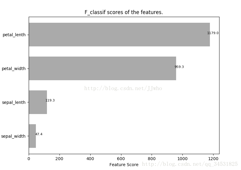

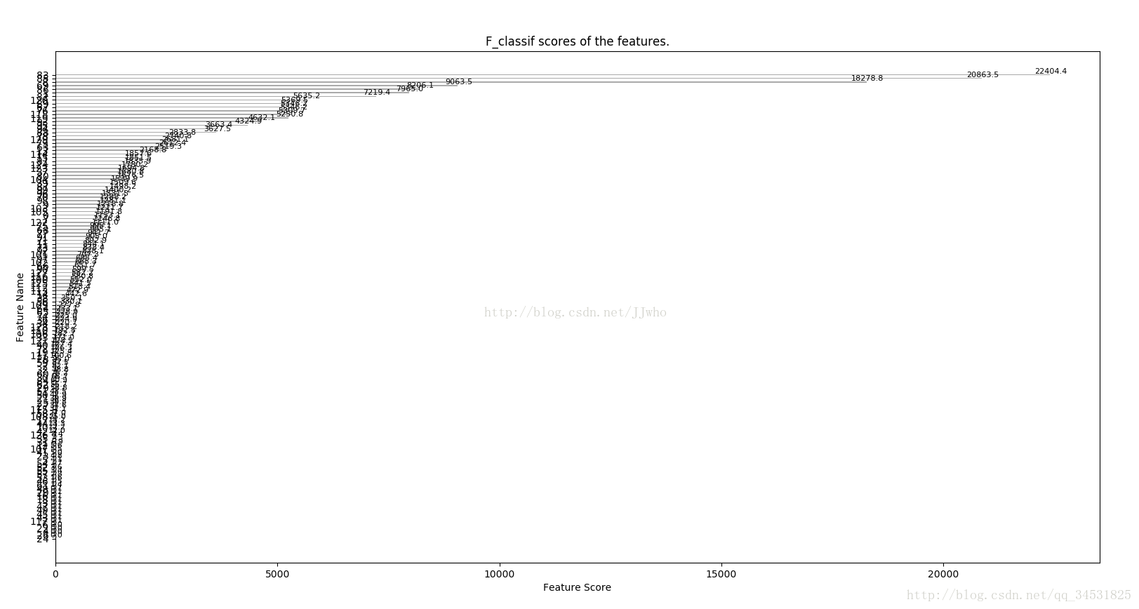
更多变量，可视化的优势就更明显了。

F检验

　　F检验又叫方差齐性检验，判断两总体方差是否相同，即方差齐性。两组数据就能得到两个S2值
F=S2/S2’。

卡方检验

　　
　　卡方检验就是统计样本的实际观测值与理论推断值之间的偏离程度，实际观测值与理论推断值之间的偏离程度就决定卡方值的大小，卡方值越大，越不符合；卡方值越小，偏差越小，越趋于符合，若两个值完全相等时，卡方值就为0，表明理论值完全符合。
　　卡方值描述了自变量与因变量之间的相关程度：卡方值越大，相关程度也越大，所以很自然的可以利用卡方值来做降维，保留相关程度大的变量。
　　

互信息

　　互信息(Mutual Information)是信息论里一种有用的信息度量，它可以看成是一个随机变量中包含的关于另一个随机变量的信息量，或者说是一个随机变量由于已知另一个随机变量而减少的不肯定性。
　　
　　

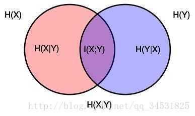
　　其中H(X)是熵，平均信息量。
　　

递归特征消除 (Recursive Feature Elimination)

RFE seeks to improve generalization performance by removing the least important features whose deletion will have the least effect on training errors.
In addition, RFE is closely related to support vector machines (SVMs) which have been shown to generalize well even for small sample classification.【３】

Feature selection using SelectFromModel

scikit learn 内容

SelectFromModel is a meta-transformer that can be used along with any estimator that has (1) a coef_ or (2) feature_importances_ attribute after fitting. The features are considered unimportant and removed, if the corresponding coef_ or feature_importances_ values are below the provided threshold parameter. Apart from specifying the threshold numerically, there are built-in heuristics for finding a threshold using a string argument. Available heuristics are “mean”, “median” and float multiples of these like “0.1*mean”.

L1-based feature selection
select the non-zero coefficients
选择非零的特征。
Tree-based feature selection
compute feature importances, which in turn can be used to discard irrelevant features.
计算特征的重要性指标，据此丢弃不相关的数据。

重要性指标

通过数据可视化发现相关性

散点图

摘自文献【４】：Python优雅地可视化数据

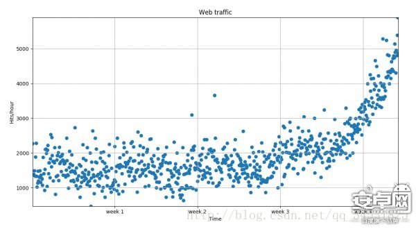
plt.scatter(x,y)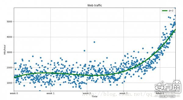

fp2 = np.polyfit(x,y,3) 
f2 = np.poly1d(fp2)  
fx = np.linspace(0,x[-1]

自定义函数的曲线拟合

import numpy as np
import matplotlib.pyplot as plt
from scipy import optimize

def fmax(x,a,b,c):
    return a*np.sin(x*np.pi/6+b)+c

x=np.arange(1,13,1)
x1=np.arange(1,13,0.1)
ymax=np.array([17, 19, 21, 28, 33, 38, 37, 37, 31, 23, 19, 18 ])

[a,b,c], _ = optimize.curve_fit(fmax,x,ymax,[1,1,1])

plt.scatter(x,ymax, color = 'black')
plt.plot(x1,fmax( x1, a, b, c ), color = 'red')
plt.show()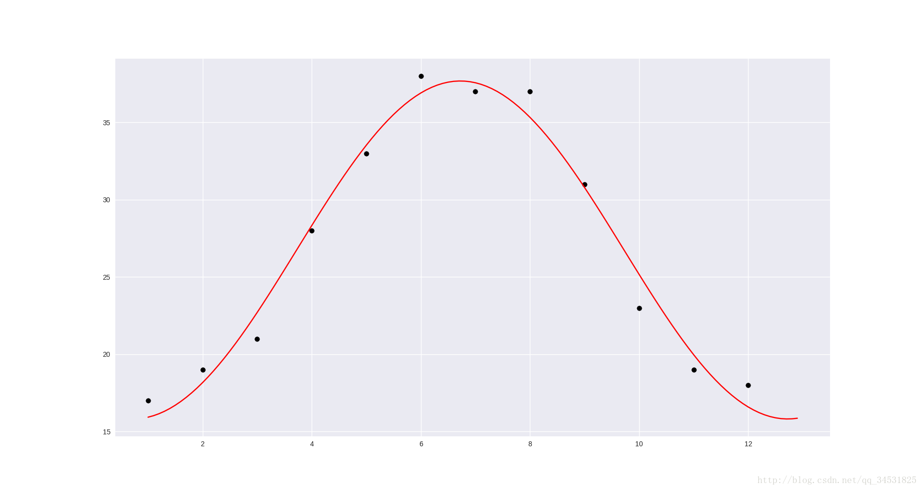

散点图矩阵　pairwise relationships

http://seaborn.pydata.org/tutorial/distributions.html#plotting-bivariate-distributions

import  seaborn  as sns
iris = sns.load_dataset("iris")
sns.pairplot(iris)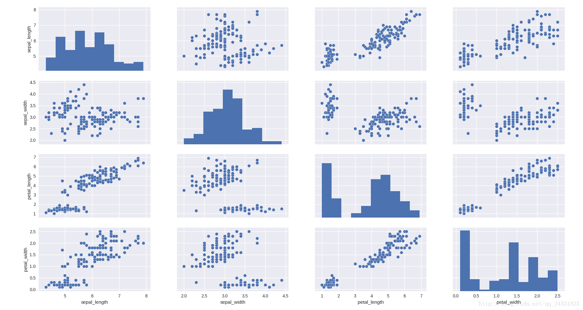

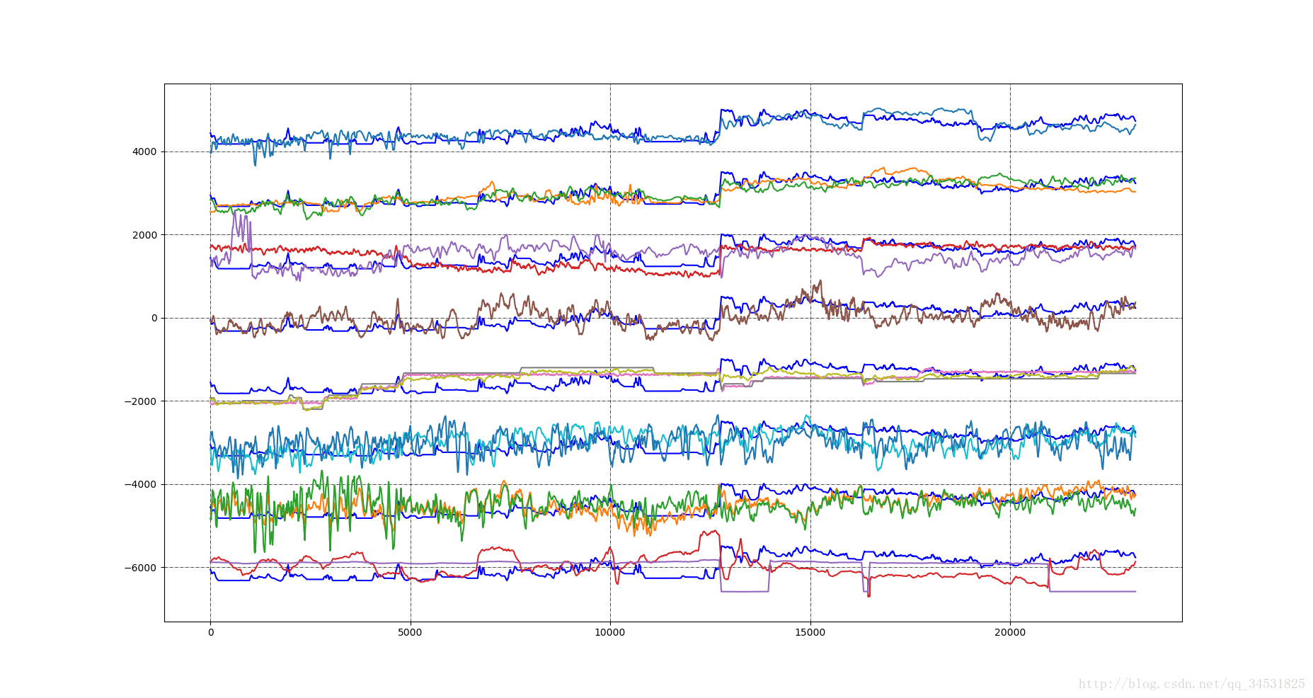
多变量折线图

热力图

http://seaborn.pydata.org/generated/seaborn.heatmap.html#seaborn.heatmap

>>> import numpy as np; np.random.seed(0)
>>> import seaborn as sns; sns.set()
>>> uniform_data = np.random.rand(10, 12)
>>> ax = sns.heatmap(uniform_data)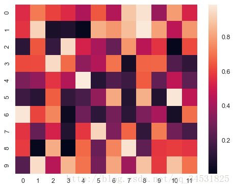

参考文献

【１】scikit-learn: http://scikit-learn.org/stable/modules/feature_selection.html

【２】https://www.cnblogs.com/stevenlk/p/6543628.html
【３】　https://www.researchgate.net/publication/4321531_Enhanced_recursive_feature_elimination　　Enhanced Recursive Feature Elimination
【４】http://news.hiapk.com/internet/s592e3e975a29.html　Python优雅地可视化数据
【５】http://blog.csdn.net/JJwho/article/details/74853549　特征选择与评分的可视化显示 - 在Python中使用Matplotlib绘制“横着的”条形图
【６】http://seaborn.pydata.org/tutorial/distributions.html#plotting-bivariate-distributions
【７】http://seaborn.pydata.org/generated/seaborn.heatmap.html#seaborn.heatmap
【８】http://blog.csdn.net/pipisorry/article/details/51695283　信息论：熵与互信息