sklearn之svm-葡萄酒质量预测(8)

class sklearn.svm.SVC(C=1.0, kernel=’rbf’, degree=3, gamma=’auto_deprecated’, coef0=0.0, shrinking=True, probability=False, tol=0.001, cache_size=200, class_weight=None, verbose=False, max_iter=-1, decision_function_shape=’ovr’, random_state=None)

C-Support向量分类。

实现基于libsvm。拟合时间复杂度大于样本数量的二次型，这使其难以扩展到包含10000个以上样本的数据集。

多类支持是根据一对一方案处理的。

核函数的精确数学公式以及gamma、coef0和degree这些参数是比较重要的

>>> linear_svc = svm.SVC(kernel='linear')
>>> linear_svc.kernel
'linear'
>>> rbf_svc = svm.SVC(kernel='rbf')
>>> rbf_svc.kernel
'rbf'

在这里插入图片描述
您可以通过将内核作为python函数或预计算Gram矩阵来定义自己的内核。

具有自定义内核的分类器与任何其他分类器的行为相同，除了:

字段support_vectors_现在为空，只有支持向量的索引存储在support_中
fit()方法中第一个参数的引用(而不是副本)被存储以供将来引用。如果这个数组在fit()和predict()的使用之间发生变化，您将会得到无法预计的结果。

使用Python函数作为内核
还可以通过在构造函数中将函数传递给关键字kernel来使用自己定义的内核。
您的内核必须以两个形状矩阵(n_samples_1, n_features)、(n_samples_2, n_features)作为参数，并返回一个形状矩阵(n_samples_1, n_samples_2)。
下面的代码定义了一个线性内核，并创建了一个使用该内核的分类器实例:

>>> import numpy as np
>>> from sklearn import svm
>>> def my_kernel(X, Y):
...     return np.dot(X, Y.T)
...
>>> clf = svm.SVC(kernel=my_kernel)

print(__doc__)

import numpy as np
import matplotlib.pyplot as plt
from sklearn import svm, datasets

# import some data to play with
iris = datasets.load_iris()
X = iris.data[:, :2]  # we only take the first two features. We could
                      # avoid this ugly slicing by using a two-dim dataset
Y = iris.target


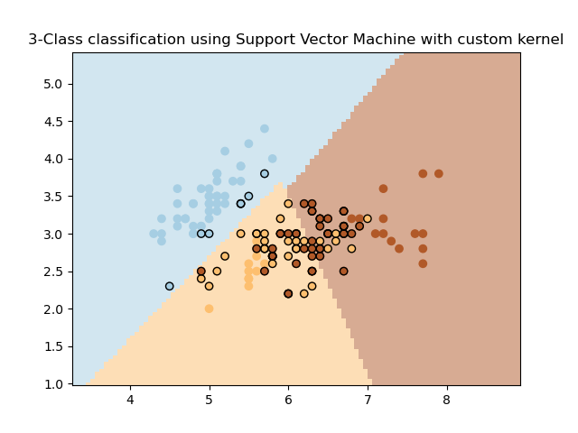
def my_kernel(X, Y):
    """
    We create a custom kernel:

                 (2  0)
    k(X, Y) = X  (    ) Y.T
                 (0  1)
    """
    M = np.array([[2, 0], [0, 1.0]])
    return np.dot(np.dot(X, M), Y.T)


h = .02  # step size in the mesh

# we create an instance of SVM and fit out data.
clf = svm.SVC(kernel=my_kernel)
clf.fit(X, Y)

# Plot the decision boundary. For that, we will assign a color to each
# point in the mesh [x_min, x_max]x[y_min, y_max].
x_min, x_max = X[:, 0].min() - 1, X[:, 0].max() + 1
y_min, y_max = X[:, 1].min() - 1, X[:, 1].max() + 1
xx, yy = np.meshgrid(np.arange(x_min, x_max, h), np.arange(y_min, y_max, h))
Z = clf.predict(np.c_[xx.ravel(), yy.ravel()])

# Put the result into a color plot
Z = Z.reshape(xx.shape)
plt.pcolormesh(xx, yy, Z, cmap=plt.cm.Paired)

# Plot also the training points
plt.scatter(X[:, 0], X[:, 1], c=Y, cmap=plt.cm.Paired, edgecolors='k')
plt.title('3-Class classification using Support Vector Machine with custom'
          ' kernel')
plt.axis('tight')
plt.show()

在这里插入图片描述
svm也可以做回归：

>>> from sklearn import svm
>>> X = [[0, 0], [2, 2]]
>>> y = [0.5, 2.5]
>>> clf = svm.SVR()
>>> clf.fit(X, y) 
SVR(C=1.0, cache_size=200, coef0=0.0, degree=3, epsilon=0.1,
    gamma='auto_deprecated', kernel='rbf', max_iter=-1, shrinking=True,
    tol=0.001, verbose=False)
>>> clf.predict([[1, 1]])
array([1.5])

print(__doc__)

import numpy as np
from sklearn.svm import SVR
import matplotlib.pyplot as plt

# #############################################################################
# Generate sample data
X = np.sort(5 * np.random.rand(40, 1), axis=0)
y = np.sin(X).ravel()

# #############################################################################
# Add noise to targets
y[::5] += 3 * (0.5 - np.random.rand(8))

# #############################################################################
# Fit regression model
svr_rbf = SVR(kernel='rbf', C=1e3, gamma=0.1)
svr_lin = SVR(kernel='linear', C=1e3)
svr_poly = SVR(kernel='poly', C=1e3, degree=2)
y_rbf = svr_rbf.fit(X, y).predict(X)
y_lin = svr_lin.fit(X, y).predict(X)
y_poly = svr_poly.fit(X, y).predict(X)

# #############################################################################
# Look at the results
lw = 2
plt.scatter(X, y, color='darkorange', label='data')
plt.plot(X, y_rbf, color='navy', lw=lw, label='RBF model')
plt.plot(X, y_lin, color='c', lw=lw, label='Linear model')
plt.plot(X, y_poly, color='cornflowerblue', lw=lw, label='Polynomial model')
plt.xlabel('data')
plt.ylabel('target')
plt.title('Support Vector Regression')
plt.legend()
plt.show()

在这里插入图片描述
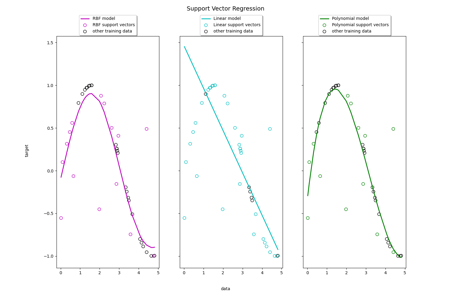
我们本例以分类为主，所以不详细涉及回归，以上2个例子是回归的简单例子，核和分类的核一样。

参数说明：
C:浮点，可选(默认=1.0)
错误项的惩罚参数C。
kernel :
内核:string，可选(默认= ’ rbf ‘)
指定算法中要使用的内核类型。它必须是‘linear’, ‘poly’, ‘rbf’, ‘sigmoid’, ‘precomputed’ ”或可调用的自定义核。如果没有给出，将使用“rbf”。如果给定一个可调用的，它将用于从数据矩阵中预先计算核矩阵;这个矩阵应该是一个形状数组(n_samples, n_samples)。
degree ：
int，可选(默认=3)
多项式核函数的次数(’ poly ')。被所有其他内核忽略。
gamma :
float，可选(默认= ’ auto ‘)
“rbf”、“poly”和“s”的核系数。
当前的默认值是“auto”，它使用1 / n_features，如果传递了gamma=‘scale’，那么它使用1 / (n_features * X.std())作为gamma的值。gamma当前的默认值“auto”将在0.22版中更改为“scale”。’ auto_deprecated ‘，作为默认值使用，表示没有传递明文值。
coef0:浮点，可选(默认=0.0)
核函数中的独立项。它只在’ poly ‘和’ s '中有意义。
shrinking : 布尔值，可选(默认=True)
是否使用收缩启发式。
probability：
概率:boolean，可选(default=False)
是否启用概率估计。这必须在调用fit之前启用，这会减慢该方法的速度。
tol:浮点型，可选(默认=1e-3)
停止criterion的错误误差。
cache_size: float，可选
指定内核缓存的大小(以MB为单位)。
class_weight: {dict， ’ balanced '}，可选
为SVC将class i的参数C设置为class_weight[i]*C。如果不给，所有的类都应该有权重1。“balanced”模式使用y值自动调整权重，与输入数据中的类频率成反比，如n_samples / (n_classes * np.bincount(y))
verbose :
bool，默认:False
启用详细输出。注意，这个设置利用了libsvm中的每个进程运行时设置，如果启用了这个设置，那么在多线程环境中可能无法正常工作。
max_iter: int，可选(默认=-1)
对求解器内迭代的硬限制，或-1为无限制。
decision_function_shape: ’ ovo '， ’ ovr ‘， default= ’ ovr ’
是否将shape (n_samples, n_classes)的one-vs-rest (’ ovr ‘)决策函数作为所有其他分类器返回，还是将libsvm中具有shape (n_samples, n_classes * (n_classes - 1) / 2)的原one-vs-one (’ ovo ')决策函数返回。
random_state: int, RandomState实例或None，可选(默认=None)
在变换数据以进行概率估计时使用的伪随机数生成器的种子。如果int, random_state为随机数生成器使用的种子;若为RandomState实例，则random_state为随机数生成器;如果没有，随机数生成器就是np.random使用的RandomState实例。

sklearn之svm-葡萄酒质量预测(8)

猜你喜欢