pandas系列学习（一）：pandas入门

作者：chen_h
微信号 & QQ：862251340
微信公众号：coderpai

介绍

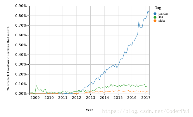
pandas 是一套用于 Python 的快速，高效的数据分析工具。近年来它的受欢迎程度飙升，与数据科学和机器学习等领域的兴起同步。

在这里插入图片描述

正如 Numpy 提供了基础的数据类型，pandas 也提供了核心数组操作，它定义了处理数据的基本结构，并且赋予了它们促进操作的方法，例如：

读取数据
调整索引
使用日期和时间序列
排序，分组，重新排序和一般数据调整
处理缺失值等等

跟复杂的统计和分析功能留给其他软件包，例如 statsmodels 和 scikit-learn，它们构建在 pandas 之上。接下来，开始我们的学习，首先我们来导入我们需要的数据包：

import pandas as pd
import numpy as np

Series

由 pandas 定义的两种重复数据类型是 Series 和 DataFrame，你可以将 Series 看做是一个 column，例如对单个变量的观察集合。DataFrame 是多个数据相关的 Series 的集合。

接下来，让我们从 Series 开始学习。

s = pd.Series(np.random.randn(4), name = "daily returns")
s

0    1.528827
1   -0.836487
2   -1.932910
3   -1.006040
Name: daily returns, dtype: float64

在这里，你可以将索引 0，1，2，3 想象成四家上市公司的索引，其对应的值是其股票的每日回报。pandas Series 是基于 numpy 阵列构建，支持许多相似的操作。

s * 100

0    152.882717
1    -83.648681
2   -193.290987
3   -100.603970
Name: daily returns, dtype: float64

np.abs(s)

0    1.528827
1    0.836487
2    1.932910
3    1.006040
Name: daily returns, dtype: float64

但是 Series 提供的不仅仅是 Numpy 数组，他们还有一些额外的方法（偏向于统计）。

s.describe()

count    4.000000
mean    -0.561652
std      1.474615
min     -1.932910
25%     -1.237757
50%     -0.921263
75%     -0.245158
max      1.528827
Name: daily returns, dtype: float64

我们还可以自定义索引的值，比如：

s.index = ['AMZN', 'AAPL', 'MSFT', 'GOOG']
s

AMZN    1.528827
AAPL   -0.836487
MSFT   -1.932910
GOOG   -1.006040
Name: daily returns, dtype: float64

通过这种方式查看，Series 就像快速，高效的 Python 词典。实际上，你可以使用与 Python 字典大致相同的语法来操作。

s['AMZN']

1.528827

s['AMZN'] = 0
s

AMZN    0.000000
AAPL   -0.836487
MSFT   -1.932910
GOOG   -1.006040
Name: daily returns, dtype: float64

'AAPL' in s

True

DataFrames

虽然 Series 非常有效，但是它是单列数据，有时候我们想处理多列数据怎么办呢？DataFrame 帮我们解决了这个问题，它是多列数据，每一列代表一个变量。实质上，pandas 中的 DataFrame 类似于（高度优化的）Excel 电子表格。因此，它是一种强大的工具，用于表示和分析自然组织成行和列的数据，通常具有针对各行和各列的描述性索引。我们来举个例子，比如我这边有一个 csv 文件，你可以点击这里下载。数据展示如下：

"country","country isocode","year","POP","XRAT","tcgdp","cc","cg"
"Argentina","ARG","2000","37335.653","0.9995","295072.21869","75.716805379","5.5788042896"
"Australia","AUS","2000","19053.186","1.72483","541804.6521","67.759025993","6.7200975332"
"India","IND","2000","1006300.297","44.9416","1728144.3748","64.575551328","14.072205773"
"Israel","ISR","2000","6114.57","4.07733","129253.89423","64.436450847","10.266688415"
"Malawi","MWI","2000","11801.505","59.543808333","5026.2217836","74.707624181","11.658954494"
"South Africa","ZAF","2000","45064.098","6.93983","227242.36949","72.718710427","5.7265463933"
"United States","USA","2000","282171.957","1","9898700","72.347054303","6.0324539789"
"Uruguay","URY","2000","3219.793","12.099591667","25255.961693","78.978740282","5.108067988"

假设你将此数据保存为当前工作目录中的 test_pwt.csv（在 Jupyter 中键入 %pwd 可以查看它是什么），我们可以按照如下形式进行读入数据：

df = pd.read_csv('https://github.com/QuantEcon/QuantEcon.lectures.code/raw/master/pandas/data/test_pwt.csv')
type(df)

pandas.core.frame.DataFrame

df

	country	country isocode	year	POP	XRAT	tcgdp	cc	cg
0	Argentina	ARG	2000	37335.653	0.999500	2.950722e+05	75.716805	5.578804
1	Australia	AUS	2000	19053.186	1.724830	5.418047e+05	67.759026	6.720098
2	India	IND	2000	1006300.297	44.941600	1.728144e+06	64.575551	14.072206
3	Israel	ISR	2000	6114.570	4.077330	1.292539e+05	64.436451	10.266688
4	Malawi	MWI	2000	11801.505	59.543808	5.026222e+03	74.707624	11.658954
5	South Africa	ZAF	2000	45064.098	6.939830	2.272424e+05	72.718710	5.726546
6	United States	USA	2000	282171.957	1.000000	9.898700e+06	72.347054	6.032454
7	Uruguay	URY	2000	3219.793	12.099592	2.525596e+04	78.978740	5.108068

我们可以使用标准的 Python 数据切片表示法选择特定的行:

df[2:5]

	country	country isocode	year	POP	XRAT	tcgdp	cc	cg
2	India	IND	2000	1006300.297	44.941600	1.728144e+06	64.575551	14.072206
3	Israel	ISR	2000	6114.570	4.077330	1.292539e+05	64.436451	10.266688
4	Malawi	MWI	2000	11801.505	59.543808	5.026222e+03	74.707624	11.658954

要选择列，我们可以传递一个列表，其中包含表示为字符串的所需列的名称：

df[['country', 'tcgdp']]

	country	tcgdp
0	Argentina	2.950722e+05
1	Australia	5.418047e+05
2	India	1.728144e+06
3	Israel	1.292539e+05
4	Malawi	5.026222e+03
5	South Africa	2.272424e+05
6	United States	9.898700e+06
7	Uruguay	2.525596e+04

要使用整数选择行和列，我们可以使用 iloc 属性，格式为 .iloc[rows, columns]

df.iloc[2:5,0:4]

	country	country isocode	year	POP
2	India	IND	2000	1006300.297
3	Israel	ISR	2000	6114.570
4	Malawi	MWI	2000	11801.505

要使用整数和标签的混合来选择行和列，我们可以以类似的方法使用 loc 属性。

df.loc[df.index[2:5], ['country', 'tcgdp']]

	country	tcgdp
2	India	1.728144e+06
3	Israel	1.292539e+05
4	Malawi	5.026222e+03

让我们想象一下，我们只关注人口和GDP（tcgdp），将数据帧 df 剥离到仅这些变量的一种方法是使用上述选择方法覆盖数据帧。

df = df[['country','POP','tcgdp']]
df

	country	POP	tcgdp
0	Argentina	37335.653	2.950722e+05
1	Australia	19053.186	5.418047e+05
2	India	1006300.297	1.728144e+06
3	Israel	6114.570	1.292539e+05
4	Malawi	11801.505	5.026222e+03
5	South Africa	45064.098	2.272424e+05
6	United States	282171.957	9.898700e+06
7	Uruguay	3219.793	2.525596e+04

这里索引 0，1，…，7 是多余的，因为我们可以使用国家名称作为索引。为此，我们将索引设置为数据框中的国家/地区变量

df = df.set_index('country')
df

	POP	tcgdp
country
Argentina	37335.653	2.950722e+05
Australia	19053.186	5.418047e+05
India	1006300.297	1.728144e+06
Israel	6114.570	1.292539e+05
Malawi	11801.505	5.026222e+03
South Africa	45064.098	2.272424e+05
United States	282171.957	9.898700e+06
Uruguay	3219.793	2.525596e+04

让我们给列取一个稍微好一点的名字

df.columns = 'population', 'total GDP'
df

	population	total GDP
country
Argentina	37335.653	2.950722e+05
Australia	19053.186	5.418047e+05
India	1006300.297	1.728144e+06
Israel	6114.570	1.292539e+05
Malawi	11801.505	5.026222e+03
South Africa	45064.098	2.272424e+05
United States	282171.957	9.898700e+06
Uruguay	3219.793	2.525596e+04

表中人口数以千计算，让我们来恢复一下，按照个计算：

df['population'] = df['population'] * 1e3
df

	population	total GDP
country
Argentina	3.733565e+07	2.950722e+05
Australia	1.905319e+07	5.418047e+05
India	1.006300e+09	1.728144e+06
Israel	6.114570e+06	1.292539e+05
Malawi	1.180150e+07	5.026222e+03
South Africa	4.506410e+07	2.272424e+05
United States	2.821720e+08	9.898700e+06
Uruguay	3.219793e+06	2.525596e+04

接下来我们将添加一个现实人均实际 GDP 的列，随着时间的推移乘以 1000000，因为总 GDP 为数百万

df['GDP percap'] = df['total GDP'] * 1e6 / df['population']
df

	population	total GDP	GDP percap
country
Argentina	3.733565e+07	2.950722e+05	7903.229085
Australia	1.905319e+07	5.418047e+05	28436.433261
India	1.006300e+09	1.728144e+06	1717.324719
Israel	6.114570e+06	1.292539e+05	21138.672749
Malawi	1.180150e+07	5.026222e+03	425.896679
South Africa	4.506410e+07	2.272424e+05	5042.647686
United States	2.821720e+08	9.898700e+06	35080.381854
Uruguay	3.219793e+06	2.525596e+04	7843.970620

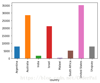
关于 pandas DataFrame 和 Series 对象的一个好处是它们具有通过 Matplotlib 工作的绘图和可视化方法。例如，我们可以轻松生成人均 GDP 的条形图。

import matplotlib.pyplot as plt

df['GDP percap'].plot(kind='bar')
plt.show()

在这里插入图片描述

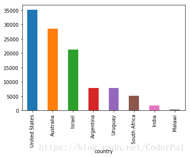
目前，数据框按照国家/地区的字母顺序排序——让我们将其改为人均 GDP。

df = df.sort_values(by='GDP percap', ascending=False)
df

	population	total GDP	GDP percap
country
United States	2.821720e+08	9.898700e+06	35080.381854
Australia	1.905319e+07	5.418047e+05	28436.433261
Israel	6.114570e+06	1.292539e+05	21138.672749
Argentina	3.733565e+07	2.950722e+05	7903.229085
Uruguay	3.219793e+06	2.525596e+04	7843.970620
South Africa	4.506410e+07	2.272424e+05	5042.647686
India	1.006300e+09	1.728144e+06	1717.324719
Malawi	1.180150e+07	5.026222e+03	425.896679

我们继续来画图:

df['GDP percap'].plot(kind='bar')
plt.show()

在这里插入图片描述