整理自唐宇迪老师的视频课程,感谢他!
本文最后会贴出所有的源代码文件,下文只是针对每个小点贴出代码进行注释说明,可以略过。
1.思路
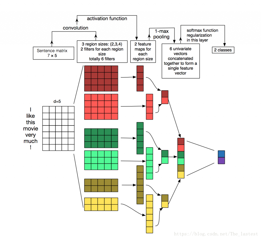
关于利用CNN做文本分类,其主要思想通过下面这幅图就能够一目了然。
本文主要记录了利用CNN来分类英文垃圾邮件的全过程。数据集主要包含两个文件:里面分别是垃圾邮件和正常邮件,用记事本就能打开。先来看看数据集长什么样:
simplistic , silly and tedious .
unfortunately the story and the actors are served with a hack script .
all the more disquieting for its relatively gore-free allusions to the serial murders , but it falls down in its attempts to humanize its subject .
a sentimental mess that never rings true .
while the performances are often engaging , this loose collection of largely improvised numbers would probably have worked better as a one-hour tv documentary .
interesting , but not compelling .
这里展示的是其中的6封邮件,可以看到每封邮件之间是通过回车换行来分隔的,我们等下也通过这个特点来分割每一个样本。
我们知道,在CNN文本分类中,是通过将每个单词对应的词向量堆叠起来,形成一个二维矩阵,以此来进行卷积和池化的。但在此处我们没有词向量怎么办呢?既然没有,那索性就不要,把它也当做一个参数,让它在训练中产生。具体做法就是:
①根据所有邮件中的单词,选取出现频率靠前的k个或者全部(本例采用全部)产生一个长度为vocabulary_size的字典(词表);
②随机初始化一个大小为[vocabulary_size,embedding_size]的词向量矩阵,embedding_size表示你用多少维的向量来表示一个词;
③对于每一封邮件,找出其每个单词在字典中对应的索引,然后按照索引从词向量矩阵中取出对应位置的词向量,堆叠形成表示该邮件的二维矩阵;
④为所有的邮件设定一个最大长度,即最多由多少个单词构成,多的截取,少的用0填充。
例如:
一封邮件内容为tomorrow is sunny,假设这三个单词在字典中对应的索引为6,2,3,且邮件的最大长度为7;那么我们首先得到这封邮件对应单词的索引序列就为:56,28,97,0,0,0,0。同时初始化的词向量矩阵为:
[[0.398 0.418 0.29  0.344 0.898 0.555 0.033 0.056 0.923]    0
 [0.668 0.957 0.428 0.942 0.692 0.084 0.413 0.619 0.02 ]    1
 [0.329 0.618 0.189 0.544 0.76  0.702 0.009 0.811 0.882]    2
 [0.912 0.042 0.777 0.765 0.708 0.887 0.944 0.272 0.5  ]    3
 [0.397 0.828 0.244 0.439 0.598 0.298 0.505 0.63  0.883]    4
 [0.402 0.084 0.419 0.66  0.69  0.031 0.354 0.117 0.494]    5
 [0.966 0.016 0.218 0.732 0.523 0.263 0.749 0.813 0.547]    6
[0.065 0.739 0.394 0.077 0.461 0.203 0.246 0.456 0.809]] 7则tomorrow is sunny这封邮件对应的矩阵就为:
[[0.966 0.016 0.218 0.732 0.523 0.263 0.749 0.813 0.547]    6
 [0.329 0.618 0.189 0.544 0.76  0.702 0.009 0.811 0.882]    2
 [0.912 0.042 0.777 0.765 0.708 0.887 0.944 0.272 0.5  ]    3
 [0.398 0.418 0.29  0.344 0.898 0.555 0.033 0.056 0.923]    0
 [0.398 0.418 0.29  0.344 0.898 0.555 0.033 0.056 0.923]    0
 [0.398 0.418 0.29  0.344 0.898 0.555 0.033 0.056 0.923]    0
 [0.398 0.418 0.29  0.344 0.898 0.555 0.033 0.056 0.923]]   0
同时,这也就对应着一个样本。可能有人就会问,初始化的词向量本来就不能表示每个词,那这样构造出来的矩阵能代表一封邮件吗?对于这个问题可以从两个角度来看:第一,开始可能它是不正确的,但由于我们这里是有监督学习,只要它不正确,最后就会会产生误差,算法可以根据产生误差来纠正这一错误,通过多次的迭代,就自然正确了;第二,虽然这个词向量矩阵是随机产生的,可能是错的,但所有邮件的表示方式都是根据这个错误的矩阵形成的,从某种意义上来说也就是对的了,我们之所以觉得它错了,是因为我们找不到一种度量方式来说明它是对的。咳,扯远了……
2 预处理
有了上面的总体思路,我们下面就细致的来对邮件进行预处理。
2.1 构造数据集
一次读入所有邮件(为一个字符串),按’\n’作为分割符分开,并去掉每个样本前后的空格。
positive = open(positive_data_file, 'rb').read().decode('utf-8')  # 得到一个字符串,因为含有中文所以加decode('utf-8')
    negative = open(negative_data_file, 'rb').read().decode('utf-8')

    positive_examples = positive.split('\n')[:-1]  # 将整个文本用换行符分割成一个一个的邮件
    negative_examples = negative.split('\n')[:-1]  # 得到的是一个list,list中的每个元素都是一封邮件(并且去掉最后一个换行符,[:-1]表示去掉最后一个元素)

    positive_examples = [s.strip() for s in positive_examples]  # 去掉每个邮件开头和结尾的的空格
    negative_examples = [s.strip() for s in negative_examples]

    x_text = positive_examples + negative_examples  # 两个列表相加构成数据集
x_text = [clean_str(sent) for sent in x_text] # 去除每个邮件中的标点等无用的字符其中函数clean_str()是去除每个样本(邮件)中的其它字符。
处理完后如下(前3个):
[“the rock is destined to be the 21st century ‘s new conan and that he ‘s going to make a splash even greater than arnold schwarzenegger , jean claud van damme or steven segal”, “the gorgeously elaborate continuation of the lord of the rings trilogy is so huge that a column of words cannot adequately describe co writer director peter jackson ‘s expanded vision of j r r tolkien ‘s middle earth”, ‘effective but too tepid biopic’]
2.2 构造标签
    positive_label = [[0, 1] for _ in positive_examples]  # 构造one-hot 标签[[0, 1], [0, 1], [0, 1], [0, 1],....]
    negative_label = [[1, 0] for _ in negative_examples]
对于每个样本,我们用One-hot的形式进行标签化处理,结果这样处理后的结果如下:
print(positive_label[:5])
[[0, 1], [0, 1], [0, 1], [0, 1], [0, 1]]
同理,负样本的标签也是如此。接着就是将两者合并到一起:
y = np.concatenate([positive_label, negative_label], axis=0)其中axis=0表示纵向堆叠,结果如下:
print(y[:5])
[[0 1]
 [0 1]
 [0 1]
 [0 1]
 [0 1]]
2.3 数字化数据集
所谓数字化数据集就是我们在第一部分中说道的,先建立一个字典,然后找到每个邮件中的单词在字典中对应的索引。好在TensorFlow已经为我们提供了这么一个模块from tensorflow.contrib import learn,让我们可以方便的得到这些。
首先我们取邮件中最长单词数作为每封邮件的长度(不足的按0填充)
max_document_length = max([len(x.split(' ')) for x in x_text])本例中max_document_length=56,也就代表着每封邮件都按56个单词处理。
接着:
vocab_processor = learn.preprocessing.VocabularyProcessor(max_document_length)
x = np.array(list(vocab_processor.fit_transform(x_text)))  # 得到每个样本中,每个单词对应在词典中的序号
print(x[:3])

#
[[ 1  2  3  4  5  6  1  7  8  9 10 11 12 13 14  9 15  5 16 17 18 19 20 21 22 23 24 25 26 27 28 29 30
0  0  0  0  0  0  0  0  0  0  0  0  0  0  0  0  0  0  0  0  0  0  0]
 [ 1 31 32 33 34  1 35 34  1 36 37  3 38 39 13 17 40 34 41 42 43 44 45 46 47 48 49  9 50 51 34 52 53 53
 54  9 55 56  0  0  0  0  0  0  0  0  0  0  0  0  0  0  0  0  0  0]
0  0  0  0  0  0  0  0  0  0  0  0  0  0  0  0  0  0  0  0  0  0]]
2.4 打乱数据并构造训练集和测试集
到目前为止,我们已经将邮件转化成了一个数字化的表现形式;但此时所有的样本都是正负样本密集聚在一起的,所有要先将其打乱。
np.random.seed(10)# 生成一个种子
shuffle_indices = np.random.permutation(np.arange(len(y)))#产生随机数
x_shuffled = x[shuffle_indices]  # 打乱数据
y_shuffled = y[shuffle_indices]

dev_sample_index = -1 * int(0.2 * float(len(y)))
x_train, x_dev = x_shuffled[:dev_sample_index], x_shuffled[dev_sample_index:]
y_train, y_dev = y_shuffled[:dev_sample_index], y_shuffled[dev_sample_index:]  # 划分训练集和验证集
此时,经过上面一系列的处理,我们已经得到了每封邮件每个单词对应的索引序列,和其对应的标签,并进行了打乱。
接着在下面一篇博文中,我们就开始进行二维矩阵的构造,然后卷积,池化全连接等。