本次所用数据来自ImageNet,使用预训练好的数据来预测一个新的数据集:猫狗图片分类。这里,使用VGG模型,这个模型内置在Keras中,直接导入就可以了。
from keras.applications import VGG16

conv_base = VGG16(weights='imagenet',
                  include_top=False,
                  input_shape=(150, 150, 3))
说一下这三个参数:
- weights:指定模型初始化权重检查点
- include_top:指定模型最后是否包含密集连接分类器。默认情况下,这个密集连接分类器对应于ImageNet的1000个类别。因为我们打算使用自己的分类器(只有两个类别:cat和dog),所以不用包含。
- input_shape:输入到网络中的图像张量(可选参数),如果不传入这个参数,那么网络可以处理任意形状的输入
看一下VGG16网络的详细构架:
conv_base.summary()
_________________________________________________________________
Layer (type)                 Output Shape              Param #
=================================================================
input_1 (InputLayer)         (None, 150, 150, 3)       0
_________________________________________________________________
block1_conv1 (Conv2D)        (None, 150, 150, 64)      1792
_________________________________________________________________
block1_conv2 (Conv2D)        (None, 150, 150, 64)      36928
_________________________________________________________________
block1_pool (MaxPooling2D)   (None, 75, 75, 64)        0
_________________________________________________________________
block2_conv1 (Conv2D)        (None, 75, 75, 128)       73856
_________________________________________________________________
block2_conv2 (Conv2D)        (None, 75, 75, 128)       147584
_________________________________________________________________
block2_pool (MaxPooling2D)   (None, 37, 37, 128)       0
_________________________________________________________________
block3_conv1 (Conv2D)        (None, 37, 37, 256)       295168
_________________________________________________________________
block3_conv2 (Conv2D)        (None, 37, 37, 256)       590080
_________________________________________________________________
block3_conv3 (Conv2D)        (None, 37, 37, 256)       590080
_________________________________________________________________
block3_pool (MaxPooling2D)   (None, 18, 18, 256)       0
_________________________________________________________________
block4_conv1 (Conv2D)        (None, 18, 18, 512)       1180160
_________________________________________________________________
block4_conv2 (Conv2D)        (None, 18, 18, 512)       2359808
_________________________________________________________________
block4_conv3 (Conv2D)        (None, 18, 18, 512)       2359808
_________________________________________________________________
block4_pool (MaxPooling2D)   (None, 9, 9, 512)         0
_________________________________________________________________
block5_conv1 (Conv2D)        (None, 9, 9, 512)         2359808
_________________________________________________________________
block5_conv2 (Conv2D)        (None, 9, 9, 512)         2359808
_________________________________________________________________
block5_conv3 (Conv2D)        (None, 9, 9, 512)         2359808
_________________________________________________________________
block5_pool (MaxPooling2D)   (None, 4, 4, 512)         0
=================================================================
Total params: 14,714,688
Trainable params: 14,714,688
Non-trainable params: 0
最后这个特征图形状为(4, 4, 512),我们在这个特征上面添加一个密集连接分类器。
不使用数据增强的快速特征提取(计算代价低)
首先,运行ImageDataGenerator实例,将图像及其标签提取为Numpy数组,调用conv_base模型的predict方法从这些图像的中提取特征。
import os
import numpy as np
from keras.preprocessing.image import ImageDataGenerator

base_dir = '/Users/fchollet/Downloads/cats_and_dogs_small'

train_dir = os.path.join(base_dir, 'train')
validation_dir = os.path.join(base_dir, 'validation')
test_dir = os.path.join(base_dir, 'test')

datagen = ImageDataGenerator(rescale=1./255)
batch_size = 20

def extract_features(directory, sample_count):
    features = np.zeros(shape=(sample_count, 4, 4, 512))
    labels = np.zeros(shape=(sample_count))
    generator = datagen.flow_from_directory(
        directory,
        target_size=(150, 150),
        batch_size=batch_size,
        class_mode='binary')
    i = 0
    for inputs_batch, labels_batch in generator:
        features_batch = conv_base.predict(inputs_batch)
        features[i * batch_size : (i + 1) * batch_size] = features_batch
        labels[i * batch_size : (i + 1) * batch_size] = labels_batch
        i += 1
        if i * batch_size >= sample_count:
            break  # 这些生成器在循环中不断生成数据,所以你必须在读完所有图像之后终止循环
    return features, labels

train_features, train_labels = extract_features(train_dir, 2000)
validation_features, validation_labels = extract_features(validation_dir, 1000)
test_features, test_labels = extract_features(test_dir, 1000)
目前,提取的特征形状为(samples, 4, 4, 512),我们要将其输入到密集连接分类器中去,所以必须首先对其形状展平为(samples ,8192)
train_features = np.reshape(train_features, (2000, 4 * 4 * 512))
validation_features = np.reshape(validation_features, (1000, 4 * 4 * 512))
test_features = np.reshape(test_features, (1000, 4 * 4 * 512))
下面定义一个密集连接分类器,并在刚刚保存好的数据和标签上训练分类器:
from keras import models
from keras import layers
from keras import optimizers

model = models.Sequential()
model.add(layers.Dense(256, activation='relu', input_dim=4 * 4 * 512))
model.add(layers.Dropout(0.5))
model.add(layers.Dense(1, activation='sigmoid'))

model.compile(optimizer=optimizers.RMSprop(lr=2e-5),
              loss='binary_crossentropy',
              metrics=['acc'])

history = model.fit(train_features, train_labels,
                    epochs=30,
                    batch_size=20,
                    validation_data=(validation_features, validation_labels))
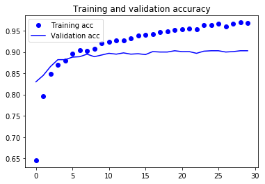
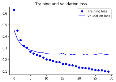
训练速度非常快,因为只需要处理两个Dense层。下面看一下训练过程中的损失曲线和精度曲线:
import matplotlib.pyplot as plt

acc = history.history['acc']
val_acc = history.history['val_acc']
loss = history.history['loss']
val_loss = history.history['val_loss']

epochs = range(len(acc))

plt.plot(epochs, acc, 'bo', label='Training acc')
plt.plot(epochs, val_acc, 'b', label='Validation acc')
plt.title('Training and validation accuracy')
plt.legend()

plt.figure()

plt.plot(epochs, loss, 'bo', label='Training loss')
plt.plot(epochs, val_loss, 'b', label='Validation loss')
plt.title('Training and validation loss')
plt.legend()

plt.show()
从图中可以看出,验证精度达到了约90%,比之前从一开始就训练小型模型效果要好很多,但是从图中也可以看出,虽然dropout比率比较大,但模型从一开始就出现了过拟合。这是因为本方法中没有使用数据增强,而数据增强对防止小型图片数据集过拟合非常重要。
使用数据增强的特征提取(计算代价高)
这种方法速度更慢,计算代价更高,但是可以在训练期间使用数据增强。这种方法是:扩展conv_base模型,然后在输入数据上端到端的运行模型。(这种方法计算代价很高,必须在GPU上运行)
承接我们之前定义的网络模型
from keras import models
from keras import layers

model = models.Sequential()
model.add(conv_base)
model.add(layers.Flatten())
model.add(layers.Dense(256, activation='relu'))
model.add(layers.Dense(1, activation='sigmoid'))
model.summary()
_________________________________________________________________
Layer (type)                 Output Shape              Param #
=================================================================
vgg16 (Model)                (None, 4, 4, 512)         14714688
_________________________________________________________________
flatten_1 (Flatten)          (None, 8192)              0
_________________________________________________________________
dense_3 (Dense)              (None, 256)               2097408
_________________________________________________________________
dense_4 (Dense)              (None, 1)                 257
=================================================================
Total params: 16,812,353
Trainable params: 16,812,353
Non-trainable params: 0
我们可以看到,VGG16的卷积基一共有14714688个参数,其上添加的分类器一共有200万个参数,非常多。
在编译和训练模型之前,需要冻结卷积基。冻结一个或多个层是指在训练过程中保持其权重不变。如果不这么做,那么卷积基之前学到的表示将会在训练过程中被修改。因为其上添加的Dense是随机初始化的,所以非常打的权重更新会在网络中进行传播,对之前学到的表示造成很大破坏。
在Keras中,冻结网络的方法是将其trainable属性设置为False
print('This is the number of trainable weights '
      'before freezing the conv base:', len(model.trainable_weights))
This is the number of trainable weights before freezing the conv base: 30
conv_base.trainable = False
print('This is the number of trainable weights '
      'after freezing the conv base:', len(model.trainable_weights))
This is the number of trainable weights after freezing the conv base: 4
如此设置之后,只有添加的两个Dense层的权重才会被训练,总共有4个权重张量,每层2个(主权重矩阵和偏置向量),注意的是,如果想修改权重属性trainable,那么应该修改好属性之后再编译模型。
下面,我们可以训练模型了,并使用数据增强的办法:
from keras.preprocessing.image import ImageDataGenerator

train_datagen = ImageDataGenerator(
      rescale=1./255,
      rotation_range=40,
      width_shift_range=0.2,
      height_shift_range=0.2,
      shear_range=0.2,
      zoom_range=0.2,
      horizontal_flip=True,
      fill_mode='nearest')

# Note that the validation data should not be augmented!
test_datagen = ImageDataGenerator(rescale=1./255)

train_generator = train_datagen.flow_from_directory(
        # This is the target directory
        train_dir,
        # All images will be resized to 150x150
        target_size=(150, 150),
        batch_size=20,
        # Since we use binary_crossentropy loss, we need binary labels
        class_mode='binary')

validation_generator = test_datagen.flow_from_directory(
        validation_dir,
        target_size=(150, 150),
        batch_size=20,
        class_mode='binary')

model.compile(loss='binary_crossentropy',
              optimizer=optimizers.RMSprop(lr=2e-5),
              metrics=['acc'])

history = model.fit_generator(
      train_generator,
      steps_per_epoch=100,
      epochs=30,
      validation_data=validation_generator,
      validation_steps=50,
      verbose=2)
model.save('cats_and_dogs_small_3.h5')
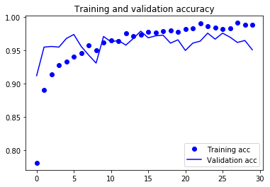
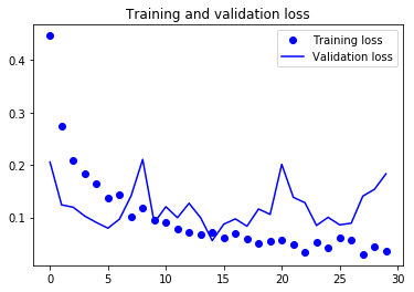
我们再来看看验证精度:
acc = history.history['acc']
val_acc = history.history['val_acc']
loss = history.history['loss']
val_loss = history.history['val_loss']

epochs = range(len(acc))

plt.plot(epochs, acc, 'bo', label='Training acc')
plt.plot(epochs, val_acc, 'b', label='Validation acc')
plt.title('Training and validation accuracy')
plt.legend()

plt.figure()

plt.plot(epochs, loss, 'bo', label='Training loss')
plt.plot(epochs, val_loss, 'b', label='Validation loss')
plt.title('Training and validation loss')
plt.legend()

plt.show()
验证精度到了将近96%,而且减少了过拟合。
微调模型
我们下面使用模型微调,进一步提高模型的性能。模型微调的步骤如下:
- (1)在已经训练好的基网络(base network)上添加自定义网络
- (2)冻结基网络
- (3)训练所添加的部分
- (4)解冻基网络的一些层
- (5)联合训练解冻的这些层和添加的部分
在做特征提取的时候已经完成了前三个步骤。我们继续第四个步骤,先解冻conv_base,然后冻结其中的部分层。
_________________________________________________________________
Layer (type)                 Output Shape              Param #
=================================================================
input_1 (InputLayer)         (None, 150, 150, 3)       0
_________________________________________________________________
block1_conv1 (Conv2D)        (None, 150, 150, 64)      1792
_________________________________________________________________
block1_conv2 (Conv2D)        (None, 150, 150, 64)      36928
_________________________________________________________________
block1_pool (MaxPooling2D)   (None, 75, 75, 64)        0
_________________________________________________________________
block2_conv1 (Conv2D)        (None, 75, 75, 128)       73856
_________________________________________________________________
block2_conv2 (Conv2D)        (None, 75, 75, 128)       147584
_________________________________________________________________
block2_pool (MaxPooling2D)   (None, 37, 37, 128)       0
_________________________________________________________________
block3_conv1 (Conv2D)        (None, 37, 37, 256)       295168
_________________________________________________________________
block3_conv2 (Conv2D)        (None, 37, 37, 256)       590080
_________________________________________________________________
block3_conv3 (Conv2D)        (None, 37, 37, 256)       590080
_________________________________________________________________
block3_pool (MaxPooling2D)   (None, 18, 18, 256)       0
_________________________________________________________________
block4_conv1 (Conv2D)        (None, 18, 18, 512)       1180160
_________________________________________________________________
block4_conv2 (Conv2D)        (None, 18, 18, 512)       2359808
_________________________________________________________________
block4_conv3 (Conv2D)        (None, 18, 18, 512)       2359808
_________________________________________________________________
block4_pool (MaxPooling2D)   (None, 9, 9, 512)         0
_________________________________________________________________
block5_conv1 (Conv2D)        (None, 9, 9, 512)         2359808
_________________________________________________________________
block5_conv2 (Conv2D)        (None, 9, 9, 512)         2359808
_________________________________________________________________
block5_conv3 (Conv2D)        (None, 9, 9, 512)         2359808
_________________________________________________________________
block5_pool (MaxPooling2D)   (None, 4, 4, 512)         0
=================================================================
Total params: 14,714,688
Trainable params: 14,714,688
Non-trainable params: 0
再回顾一下这些层,我们将微调最后三个卷积层,也就是说,知道block4_pool的所有层都应该被冻结,后面三层来进行训练。
要知道,训练的参数越多,过拟合的风险越大。卷积基有1500万个参数,所以你在小型数据集上训练这么多参数是有风险的。因此,这种情况下最好的策略是仅微调卷积基最后三两层。
conv_base.trainable = True

set_trainable = False
for layer in conv_base.layers:
    if layer.name == 'block5_conv1':
        set_trainable = True
    if set_trainable:
        layer.trainable = True
    else:
        layer.trainable = False
现在可以微调网络了,我们将使用学习率非常小的RMSProp优化器来实现。之所以让学习率很小,是因为对于微调网络的三层表示,我们希望其变化范围不要太大,太大的权重可能会破坏这些表示。
model.compile(loss='binary_crossentropy',
              optimizer=optimizers.RMSprop(lr=1e-5),
              metrics=['acc'])

history = model.fit_generator(
      train_generator,
      steps_per_epoch=100,
      epochs=100,
      validation_data=validation_generator,
      validation_steps=50)
model.save('cats_and_dogs_small_4.h5')
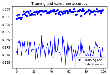
下面,绘制曲线看看效果:
acc = history.history['acc']
val_acc = history.history['val_acc']
loss = history.history['loss']
val_loss = history.history['val_loss']
epochs = range(len(acc))
plt.plot(epochs, acc, 'bo', label='Training acc')
plt.plot(epochs, val_acc, 'b', label='Validation acc')
plt.title('Training and validation accuracy')
plt.legend()
plt.figure()
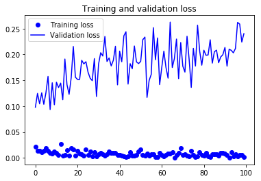
plt.plot(epochs, loss, 'bo', label='Training loss')
plt.plot(epochs, val_loss, 'b', label='Validation loss')
plt.title('Training and validation loss')
plt.legend()
plt.show()
这些曲线看起来包含噪音。为了让图像更具有可读性,可以让每个损失精度替换为指数移动平均,从而让曲线变得更加平滑,下面用一个简单实用函数来实现:
def smooth_curve(points, factor=0.8):
  smoothed_points = []
  for point in points:
    if smoothed_points:
      previous = smoothed_points[-1]
      smoothed_points.append(previous * factor + point * (1 - factor))
    else:
      smoothed_points.append(point)
  return smoothed_points

plt.plot(epochs,
         smooth_curve(acc), 'bo', label='Smoothed training acc')
plt.plot(epochs,
         smooth_curve(val_acc), 'b', label='Smoothed validation acc')
plt.title('Training and validation accuracy')
plt.legend()

plt.figure()

plt.plot(epochs,
         smooth_curve(loss), 'bo', label='Smoothed training loss')
plt.plot(epochs,
         smooth_curve(val_loss), 'b', label='Smoothed validation loss')
plt.title('Training and validation loss')
plt.legend()

plt.show()
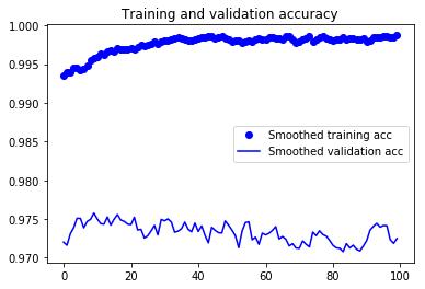

通过指数移动平均,验证曲线变得更清楚了。可以看到,精度提高了1%,约从96%提高到了97%。
下面,在测试集上评估一下这个模型
test_generator = test_datagen.flow_from_directory(
        test_dir,
        target_size=(150, 150),
        batch_size=20,
        class_mode='binary')

test_loss, test_acc = model.evaluate_generator(test_generator, steps=50)
print('test acc:', test_acc)
Found 1000 images belonging to 2 classes.
test acc: 0.967999992371
得到了差不多97%的测试精度,在关于这个数据集的原始Kaggle竞赛中,这个结果是最佳结果之一。
值得注意的是,我们只是用了一小部分训练数据(约10%)就得到了这个结果。训练20000个样本和训练2000个样本还是有很大差别的。
更多精彩内容,欢迎关注我的微信公众号:数据瞎分析