基于TensorFlow的SSD车辆检测-2

版权声明：本文为博主原创文章，转载请注明出处 https://blog.csdn.net/shuzfan/article/details/79791116

此系列博客是用来学习Tensorflow和Python的，由于是新手上车，如有错误之处希望大家不吝指出。

整个项目可以从百度云下载：链接：https://pan.baidu.com/s/1f2JPJpE7m5M2kSifMP0-Lw 密码：9p8v

二. SSD网络构建

在网络模型构建环节，主要包含下面三块内容：

• 构建网络的基础部分：VGG_base
• 构建网络的分支部分：SSD的6个预测分支
• SSD的loss设计

SSD的网络结构如下所示，后面的讲解基本就按照该模型来。

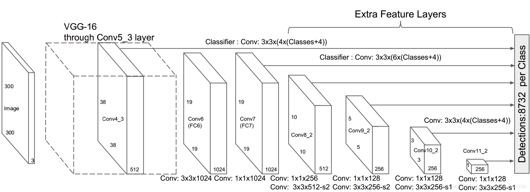
1. VGG_base构建

SSD基础部分采用了VGG16的部分结构：

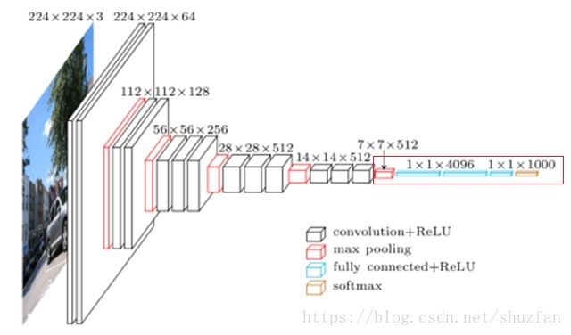
实现的主要区别有：
- （1）舍弃上图红框中的结构，只保留卷积部分；
- （2）本博客实现的是SSD-300，而原来的VGG16的输入是224x224；
- （3）此外，尽量使用pre-trained的VGG16模型来初始话我们的VGG-base;

具体实现如下：

# coding=utf-8

""" vgg_base.py:
    To build the basic VGG16 part of the SSD net.
    The input shape is n*300*300*3
"""

import tensorflow as tf

VGG_MEAN = [103.939, 116.779, 123.68]


def vgg_net(images):
    with tf.name_scope('VGG_base'):

        # zero-mean input
        mean = tf.constant([123.68, 116.779, 103.939], dtype=tf.float32, shape=[1, 1, 1, 3], name='img_mean')
        inputs = images - mean

        # build the vgg16 net
        # block1, the output is 150*150*64
        conv1_1 = conv_layer(inputs, 64, 'conv1_1')
        conv1_2 = conv_layer(conv1_1, 64, 'conv1_2')
        pool1 = max_pooling_layer(conv1_2, 'pool1')

        # block2, the output is 75*75*128
        conv2_1 = conv_layer(pool1, 128, 'conv2_1')
        conv2_2 = conv_layer(conv2_1, 128, 'conv2_2')
        pool2 = max_pooling_layer(conv2_2, 'pool2')

        # block3, the output is 38*38*256
        conv3_1 = conv_layer(pool2, 256, 'conv3_1')
        conv3_2 = conv_layer(conv3_1, 256, 'conv3_2')
        conv3_3 = conv_layer(conv3_2, 256, 'conv3_3')
        pool3 = max_pooling_layer(conv3_3, 'pool3')

        # block4, the output is 19*19*512
        conv4_1 = conv_layer(pool3,512, 'conv4_1')
        conv4_2 = conv_layer(conv4_1, 512, 'conv4_2')
        conv4_3 = conv_layer(conv4_2, 512, 'conv4_3')
        pool4 = max_pooling_layer(conv4_3, 'pool4')

        # block5,no pooling, the output is 19*19*512
        conv5_1 = conv_layer(pool4, 512, 'conv5_1')
        conv5_2 = conv_layer(conv5_1, 512, 'conv5_2')
        conv5_3 = conv_layer(conv5_2, 512, 'conv5_3')

        return conv4_3, conv5_3


# convolution layer, the default kernel size is 3, the default stride is 1
def conv_layer(inputs, num_output, name=None):
    # get the number of channels of the inputs
    num_input = inputs.get_shape()[-1].value
    with tf.name_scope(name):
        weights = tf.get_variable(name + '_w',
                                  shape=[3, 3, num_input, num_output],
                                  dtype=tf.float32,
                                  initializer=tf.glorot_normal_initializer())

        conv = tf.nn.conv2d(inputs, weights, [1, 1, 1, 1], padding='SAME')

        bias = tf.get_variable(name + '_b',
                               shape=[num_output],
                               dtype=tf.float32,
                               initializer=tf.constant_initializer(0))
        conv_b = tf.nn.bias_add(conv, bias)
        conv_b = tf.nn.relu(conv_b)
        return conv_b


# max-pooling layer, the default kernel size is 2, the default stride is 2
def max_pooling_layer(inputs, name):
    return tf.nn.max_pool(inputs, ksize=[1, 2, 2, 1], strides=[1, 2, 2, 1], padding='SAME', name=name)

另外，在util.py中实现了VGG_base使用pre-trained模型的方法：
（该模型参数存放于net文件夹下的vgg_base.npz文件中）

# util.py

# coding=utf-8

import numpy as np
import tensorflow as tf


# initiate the parameters of vgg_net from a pre-trained model
def load_vgg_weights(sess, vgg_model_path=None):
    if vgg_model_path is None:
        print('Init VGG16 base model with random variables.')
    else:
        weights = np.load(vgg_model_path)
        keys = sorted(weights.keys())
        with tf.variable_scope('', reuse=True):
            for key in keys:
                sess.run(tf.get_variable(key).assign(weights[key]))
        print('Init VGG16 base model from pre-trained weights.')

2. SSD的6个分支

SSD的6个分支部分其结构如下图所示：

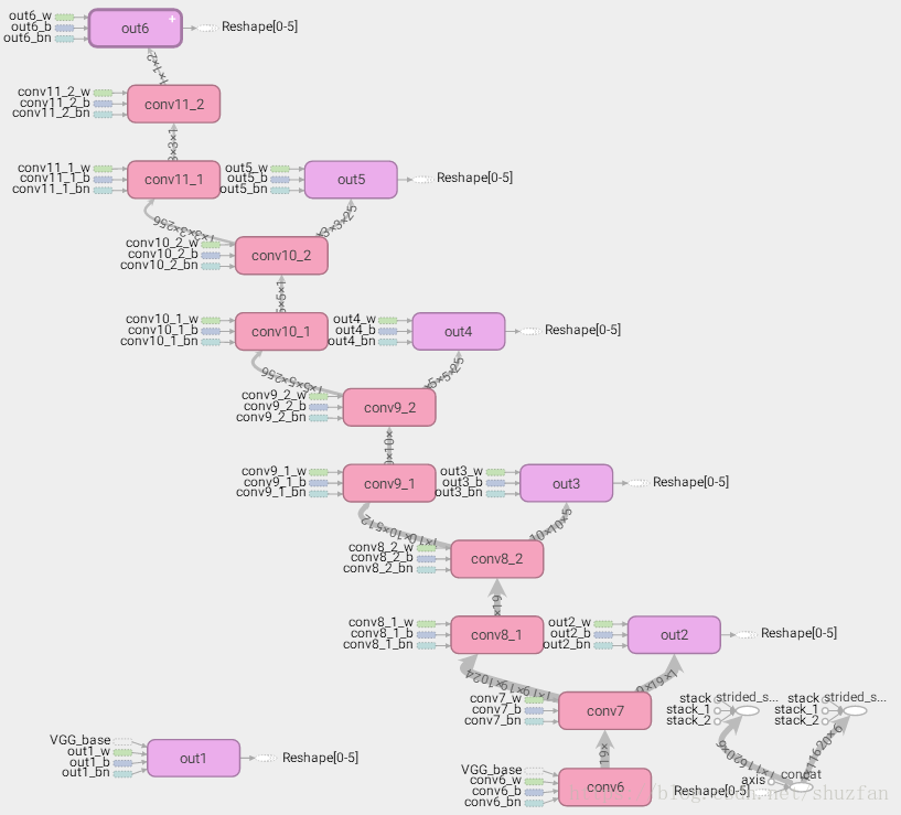
实现时的注意事项主要有：

• （1）为了加快训练，在卷积层后引入了Batch Normalization。关于BN的实现可参照https://blog.csdn.net/shuzfan/article/details/79054561；
• （2）由于最后一个卷积层用于做分类和bounding box回归，因此该卷积层后不再使用ReLU激活函数；
• （3）该部分网络结构基本与论文保持一致。注意conv10和conv11卷积时的边缘补齐方式；
• （4）关于预测层的anchor的数量与论文原文略有不同，这一细节会在后续的第三章介绍；

最终该部分实现如下：

# coding=utf-8

# build the complete SSD net based on VGG16

import tensorflow as tf
from net.vgg_base import vgg_net
from data.constants import *


def ssd(images, is_training):

    # stop gradient to images
    images = tf.stop_gradient(images)
    # build the vgg16
    vgg16_conv4_3, vgg16_conv5_3 = vgg_net(images)

    # build the extension part of SSD net
    with tf.name_scope('ssd_ext'):
        # block6 the output is 19*19*1024
        conv6 = conv_bn_layer('conv6', vgg16_conv5_3, is_training, 1024, 3, 1)

        # block7 the output is 19*19*1024
        conv7 = conv_bn_layer('conv7', conv6, is_training, 1024, 1, 1)

        # block8 the output is 为10*10*512
        conv8_1 = conv_bn_layer('conv8_1', conv7, is_training, 256, 1, 1)
        conv8_2 = conv_bn_layer('conv8_2', conv8_1, is_training, 512, 3, 2)

        # block9 the output is 5*5*256
        conv9_1 = conv_bn_layer('conv9_1', conv8_2, is_training, 128, 1, 1)
        conv9_2 = conv_bn_layer('conv9_2', conv9_1, is_training, 256, 3, 2)

        # block10 then output is 3*3*256
        conv10_1 = conv_bn_layer('conv10_1', conv9_2, is_training, 128, 1, 1)
        conv10_2 = conv_bn_layer('conv10_2', conv10_1, is_training, 256, 3, 1, m_padding='VALID')

        # block11 the output is 1*1*256
        conv11_1 = conv_bn_layer('conv11_1', conv10_2, is_training, 128, 1, 1)
        conv11_2 = conv_bn_layer('conv11_2', conv11_1, is_training, 256, 3, 1, m_padding='VALID')

        # prediction layers
        out1 = conv_bn_layer('out1', vgg16_conv4_3, is_training, anchors_num[0]*(2+4), 3, 1, is_act=False)
        out2 = conv_bn_layer('out2', conv7, is_training, anchors_num[1]*(2+4), 3, 1, is_act=False)
        out3 = conv_bn_layer('out3', conv8_2, is_training, anchors_num[2]*(2+4), 3, 1, is_act=False)
        out4 = conv_bn_layer('out4', conv9_2, is_training, anchors_num[3]*(2+4), 3, 1, is_act=False)
        out5 = conv_bn_layer('out5', conv10_2, is_training, anchors_num[4]*(2+4), 3, 1, is_act=False)
        out6 = conv_bn_layer('out6', conv11_2, is_training, anchors_num[5]*(2+4), 1, 1, is_act=False)

        # reshape the  outputs
        out1 = tf.reshape(out1, [-1, feature_size[0] * feature_size[0] * anchors_num[0], 6])
        out2 = tf.reshape(out2, [-1, feature_size[1] * feature_size[1] * anchors_num[1], 6])
        out3 = tf.reshape(out3, [-1, feature_size[2] * feature_size[2] * anchors_num[2], 6])
        out4 = tf.reshape(out4, [-1, feature_size[3] * feature_size[3] * anchors_num[3], 6])
        out5 = tf.reshape(out5, [-1, feature_size[4] * feature_size[4] * anchors_num[4], 6])
        out6 = tf.reshape(out6, [-1, feature_size[5] * feature_size[5] * anchors_num[5], 6])

        # concat all predictions from six detection branches
        outputs = tf.concat([out1, out2, out3, out4, out5, out6], 1)

        # slice
        cls_predict = outputs[:, :, :2]
        reg_predict = outputs[:, :, 2:]

        return cls_predict, reg_predict


# the defination of convolution layer
def conv_bn_layer(name, bottom, is_training, num_output,
                  kernel_size, stride, is_bn=True, is_act=True, m_padding='SAME'):
    bottom = tf.convert_to_tensor(bottom)
    num_input = bottom.get_shape()[-1].value
    with tf.name_scope(name):
        weights = tf.get_variable(name+'_w',
                                  shape=[kernel_size, kernel_size, num_input, num_output],
                                  dtype=tf.float32,
                                  initializer=tf.glorot_normal_initializer())
        conv = tf.nn.conv2d(bottom, weights, [1, stride, stride, 1], padding=m_padding)

        bias = tf.get_variable(name + '_b',
                               shape=[num_output],
                               dtype=tf.float32,
                               initializer=tf.constant_initializer(0))

        conv_b = tf.nn.bias_add(conv, bias)

        # whether use Batch Normalization
        if is_bn is True:
            conv_b = bn_layer(conv_b, is_training, name=name+'_bn')

        # whether use ReLU activation
        if is_act is True:
            conv_b = tf.nn.relu(conv_b, name=name+'_relu')

        return conv_b


# the defination of batch normalization layer
def bn_layer(x, is_training, name='BatchNorm', moving_decay=0.9, eps=1e-5):
    # assert whether fitting a convolutional layer (4) or a fully-connected layer (2)
    shape = x.shape
    assert len(shape) in [2, 4]

    param_shape = shape[-1]
    with tf.variable_scope(name):
        gamma = tf.get_variable(name+'_gamma', param_shape, initializer=tf.constant_initializer(1))
        beta = tf.get_variable(name+'_beat', param_shape, initializer=tf.constant_initializer(0))

        # compute present means and variances
        axes = list(range(len(shape)-1))
        batch_mean, batch_var = tf.nn.moments(x, axes, name='moments')

        # update the means and variances by moving average method
        ema = tf.train.ExponentialMovingAverage(moving_decay)

        def mean_var_with_update():
            ema_apply_op = ema.apply([batch_mean, batch_var])
            with tf.control_dependencies([ema_apply_op]):
                return tf.identity(batch_mean), tf.identity(batch_var)

        # when training, update the means and variances; when testing, use the history results
        mean, var = tf.cond(tf.equal(is_training, True), mean_var_with_update,
                            lambda: (ema.average(batch_mean), ema.average(batch_var)))

        return tf.nn.batch_normalization(x, mean, var, beta, gamma, eps,name=name)

3. SSD的loss设计

SSD原文中的loss函数如下：

该loos主要有以下特点：

（1）回归任务只针对匹配成功的anchor，且使用smooth L1 loss:

具体实现如下：

# compute the smooth_l1 loss
def smooth_l1(x):
    # L1
    l1 = tf.abs(x) - 0.5
    # L2
    l2 = 0.5 * (x**2.0)
    # find abs(x_i) < 1
    condition = tf.less(tf.abs(x), 1.0)

    return tf.where(condition, l2, l1)

（2）N 表示成功匹配的anchor数量，当N=0时整个loss直接置为0

（3）为保证训练样本的均衡：通过对背景区域anchor的loss进行排序并选中其中最难的一批来保证总的正负样本比例为1：3

大概的实现如下：（注意这个函数，本人没有测试过）

# the loss function of SSD Model
# cls_predict is the prediction tensor for classification whose shape is batch_size*8732*2
# reg_predict is the prediction tensor for regression whose shape is batch_size*8732*4
def ssd_loss(cls_predict, reg_predict, cls_label, reg_label,
             negpos_ratio=3, alpha=1.0, scope='ssd_loss'):
    with tf.name_scope(scope):

        # convert to tensor
        cls_label = tf.convert_to_tensor(cls_label, dtype=tf.float32)
        reg_label = tf.convert_to_tensor(reg_label, dtype=tf.float32)

        mean_cls_loss = tf.zeros([1], dtype=tf.float32)
        mean_reg_loss = tf.zeros([1], dtype=tf.float32)
        mean_all_loss = tf.zeros([1], dtype=tf.float32)

        batch = cls_label.get_shape()[-1].value

        # process images iteratively
        for i in range(batch):
            # find all positive examples and negative examples separately
            pos_mask = cls_label[i, :, 1] > 0.5
            pos_mask = tf.reshape(pos_mask, [all_anchors_num, 1])
            neg_mask = tf.logical_not(pos_mask)

            # compute the number of positives
            pos_mask = tf.cast(pos_mask, tf.float32)
            pos_num = tf.reduce_sum(pos_mask)

            # if pos_num is zero
            pos_num = tf.where(pos_num > 0, pos_num, 1)

            # hard mining, the number of adopted negative examples
            neg_num = tf.minimum(pos_num*negpos_ratio, all_anchors_num-pos_num)

            # find negative examples with top_k loss
            neg_prob = tf.nn.softmax(cls_predict[i, :, :])
            neg_prob = tf.reshape(neg_prob[:, 1], [all_anchors_num, 1])
            neg_prob = tf.where(neg_mask, neg_prob, tf.zeros(neg_mask.shape, dtype=tf.float32))
            val, indexes = tf.nn.top_k(neg_prob, k=tf.cast(neg_num, tf.int32))
            neg_mask = neg_prob > val[-1]
            neg_mask = tf.cast(neg_mask, tf.float32)

            # compute all loss
            anchor_cls_loss = tf.nn.softmax_cross_entropy_with_logits_v2(labels=cls_label[i, :, :],
                                                                         logits=cls_predict[i, :, :])
            anchor_reg_loss = smooth_l1(reg_predict[i, :, :] - reg_label[i, :, :])

            # weighted loss
            cls_loss = tf.losses.compute_weighted_loss(anchor_cls_loss, pos_mask+neg_mask)
            cls_loss = tf.reduce_sum(cls_loss) / pos_num
            reg_loss = tf.losses.compute_weighted_loss(anchor_reg_loss, pos_mask)
            reg_loss = tf.reduce_sum(reg_loss) / pos_num

            # add the losses and compute the mean
            mean_cls_loss += (cls_loss / batch)
            mean_reg_loss += (reg_loss / batch)
            mean_all_loss += (cls_loss + alpha*reg_loss) / batch

        return mean_cls_loss, mean_reg_loss, mean_all_loss

对于使用KITTI数据集进行车辆检测而言，SSD原始的分类loss有以下缺点：

• (1) KITTI中有些图片没有车辆，此时如果按照原始的SSD分类loss，则会因为N=0而直接将loss置为0，则导致图片无法被利用。
• (2) 通过在线将loss进行排序来选择负样本来保证正负样本比例为1:3的做法比较慢。

因此，个人针对上述问题设计了一个新的loss:

该loss的核心在于在准备图片阶段提前准备好用于分类和回归任务的加权mask，具体地：

（1）举例比如一共有K=10个anchors，其中正样本为N=2个，则负样本为M=8个。我们用于分类的label为[1, 0, 1, 0, 0, 0, 0, 0, 0, 0]。

（2）当N>0时，则正样本分类的加权mask为：pos_mask=[1, 0, 1, 0, 0, 0, 0, 0, 0, 0] / N = [0.5, 0, 0.5, 0, 0, 0, 0, 0, 0, 0]。

（3）当M>0时，且设定正负样本比例为1：3时，则负样本分类的加权mask为：neg_mask={1-[1, 0, 1, 0, 0, 0, 0, 0, 0, 0]} / M * 3 = [0, 0.375, 0, 0.375, 0.375, 0.375, 0.375, 0.375, 0.375, 0.375]。

(4) 然后整个分类任务的加权mask为：cls_mask = pos_mask + neg_mask = [0.5, 0.375, 0.5, 0.375, 0.375, 0.375, 0.375, 0.375, 0.375, 0.375]

(5) 假设回归任务的权重系数为alpha， 则回归任务的加权mask为：reg_mask = pos_mask * alpha

当有了上述的mask时，我们SSD的新loss如下：

# my new loss function of SSD Model
# cls_predict is the prediction tensor for classification whose shape is batch_size*8732*2
# reg_predict is the prediction tensor for regression whose shape is batch_size*8732*4
def ssd_loss_new(cls_predict, reg_predict, cls_label, reg_label,
                 cls_mask, reg_mask, scope='ssd_loss_new'):
    with tf.name_scope(scope):

        # stop gradients to labels
        cls_label = tf.stop_gradient(cls_label)
        reg_label = tf.stop_gradient(reg_label)
        cls_mask = tf.stop_gradient(cls_mask)
        reg_mask = tf.stop_gradient(reg_mask)

        batch = cls_predict.get_shape()[0].value

        cls_predict = tf.reshape(cls_predict, [batch * all_anchors_num, 2])
        reg_predict = tf.reshape(reg_predict, [batch * all_anchors_num, 4])
        # cls_label = tf.reshape(cls_label, [batch*all_anchors_num, 2])
        # reg_label = tf.reshape(reg_label, [batch * all_anchors_num, 4])

        # compute all loss
        cls_loss = tf.nn.softmax_cross_entropy_with_logits(labels=cls_label, logits=cls_predict)
        reg_loss = tf.reduce_sum(smooth_l1(reg_predict - reg_label), 1)

        # mask
        cls_loss = tf.reduce_sum(tf.multiply(cls_loss, cls_mask)) / batch
        reg_loss = tf.reduce_sum(tf.multiply(reg_loss, reg_mask)) / batch

        return cls_loss, reg_loss, cls_loss + reg_loss