Skip to content
Features
Business
Explore
Marketplace
Pricing

Search

Sign in or Sign up
 Watch 2,591  Star 41,709  Fork 24,991 tensorflow/models
 Code  Issues 1,041  Pull requests 286  Projects 2  Wiki  Insights
Dismiss
Join GitHub today
GitHub is home to over 28 million developers working together to host and review code, manage projects, and build software together.

Sign up
Branch: master Find file Copy path models/tutorials/image/cifar10/cifar10_input.py
e1ac09e  on 13 Jan
@StevenHickson StevenHickson Updated cifar10_input.py to put the data augmentation into a name_sco…
6 contributors @nealwu @itsmeolivia @mrphoenix13 @StevenHickson @jihobak @aselle
RawBlameHistory     
262 lines (209 sloc)  9.97 KB
# Copyright 2015 The TensorFlow Authors. All Rights Reserved.
#
# Licensed under the Apache License, Version 2.0 (the "License");
# you may not use this file except in compliance with the License.
# You may obtain a copy of the License at
#
#     http://www.apache.org/licenses/LICENSE-2.0
#
# Unless required by applicable law or agreed to in writing, software
# distributed under the License is distributed on an "AS IS" BASIS,
# WITHOUT WARRANTIES OR CONDITIONS OF ANY KIND, either express or implied.
# See the License for the specific language governing permissions and
# limitations under the License.
# ==============================================================================

"""Routine for decoding the CIFAR-10 binary file format."""

from __future__ import absolute_import
from __future__ import division
from __future__ import print_function

import os

from six.moves import xrange  # pylint: disable=redefined-builtin
import tensorflow as tf

# Process images of this size. Note that this differs from the original CIFAR
# image size of 32 x 32. If one alters this number, then the entire model
# architecture will change and any model would need to be retrained.
IMAGE_SIZE = 24

# Global constants describing the CIFAR-10 data set.
NUM_CLASSES = 10
NUM_EXAMPLES_PER_EPOCH_FOR_TRAIN = 50000
NUM_EXAMPLES_PER_EPOCH_FOR_EVAL = 10000


def read_cifar10(filename_queue):
  """Reads and parses examples from CIFAR10 data files.
  Recommendation: if you want N-way read parallelism, call this function
  N times.  This will give you N independent Readers reading different
  files & positions within those files, which will give better mixing of
  examples.
  Args:
    filename_queue: A queue of strings with the filenames to read from.
  Returns:
    An object representing a single example, with the following fields:
      height: number of rows in the result (32)
      width: number of columns in the result (32)
      depth: number of color channels in the result (3)
      key: a scalar string Tensor describing the filename & record number
        for this example.
      label: an int32 Tensor with the label in the range 0..9.
      uint8image: a [height, width, depth] uint8 Tensor with the image data
  """

  class CIFAR10Record(object):
    pass
  result = CIFAR10Record()

  # Dimensions of the images in the CIFAR-10 dataset.
  # See http://www.cs.toronto.edu/~kriz/cifar.html for a description of the
  # input format.
  label_bytes = 1  # 2 for CIFAR-100
  result.height = 32
  result.width = 32
  result.depth = 3
  image_bytes = result.height * result.width * result.depth
  # Every record consists of a label followed by the image, with a
  # fixed number of bytes for each.
  record_bytes = label_bytes + image_bytes

  # Read a record, getting filenames from the filename_queue.  No
  # header or footer in the CIFAR-10 format, so we leave header_bytes
  # and footer_bytes at their default of 0.
  reader = tf.FixedLengthRecordReader(record_bytes=record_bytes)
  result.key, value = reader.read(filename_queue)

  # Convert from a string to a vector of uint8 that is record_bytes long.
  record_bytes = tf.decode_raw(value, tf.uint8)

  # The first bytes represent the label, which we convert from uint8->int32.
  result.label = tf.cast(
      tf.strided_slice(record_bytes, [0], [label_bytes]), tf.int32)

  # The remaining bytes after the label represent the image, which we reshape
  # from [depth * height * width] to [depth, height, width].
  depth_major = tf.reshape(
      tf.strided_slice(record_bytes, [label_bytes],
                       [label_bytes + image_bytes]),
      [result.depth, result.height, result.width])
  # Convert from [depth, height, width] to [height, width, depth].
  result.uint8image = tf.transpose(depth_major, [1, 2, 0])

  return result


def _generate_image_and_label_batch(image, label, min_queue_examples,
                                    batch_size, shuffle):
  """Construct a queued batch of images and labels.
  Args:
    image: 3-D Tensor of [height, width, 3] of type.float32.
    label: 1-D Tensor of type.int32
    min_queue_examples: int32, minimum number of samples to retain
      in the queue that provides of batches of examples.
    batch_size: Number of images per batch.
    shuffle: boolean indicating whether to use a shuffling queue.
  Returns:
    images: Images. 4D tensor of [batch_size, height, width, 3] size.
    labels: Labels. 1D tensor of [batch_size] size.
  """
  # Create a queue that shuffles the examples, and then
  # read 'batch_size' images + labels from the example queue.
  num_preprocess_threads = 16
  if shuffle:
    images, label_batch = tf.train.shuffle_batch(
        [image, label],
        batch_size=batch_size,
        num_threads=num_preprocess_threads,
        capacity=min_queue_examples + 3 * batch_size,
        min_after_dequeue=min_queue_examples)
  else:
    images, label_batch = tf.train.batch(
        [image, label],
        batch_size=batch_size,
        num_threads=num_preprocess_threads,
        capacity=min_queue_examples + 3 * batch_size)

  # Display the training images in the visualizer.
  tf.summary.image('images', images)

  return images, tf.reshape(label_batch, [batch_size])


def distorted_inputs(data_dir, batch_size):
  """Construct distorted input for CIFAR training using the Reader ops.
  Args:
    data_dir: Path to the CIFAR-10 data directory.
    batch_size: Number of images per batch.
  Returns:
    images: Images. 4D tensor of [batch_size, IMAGE_SIZE, IMAGE_SIZE, 3] size.
    labels: Labels. 1D tensor of [batch_size] size.
  """
  filenames = [os.path.join(data_dir, 'data_batch_%d.bin' % i)
               for i in xrange(1, 6)]
  for f in filenames:
    if not tf.gfile.Exists(f):
      raise ValueError('Failed to find file: ' + f)

  # Create a queue that produces the filenames to read.
  filename_queue = tf.train.string_input_producer(filenames)

  with tf.name_scope('data_augmentation'):
    # Read examples from files in the filename queue.
    read_input = read_cifar10(filename_queue)
    reshaped_image = tf.cast(read_input.uint8image, tf.float32)

    height = IMAGE_SIZE
    width = IMAGE_SIZE

    # Image processing for training the network. Note the many random
    # distortions applied to the image.

    # Randomly crop a [height, width] section of the image.
    distorted_image = tf.random_crop(reshaped_image, [height, width, 3])

    # Randomly flip the image horizontally.
    distorted_image = tf.image.random_flip_left_right(distorted_image)

    # Because these operations are not commutative, consider randomizing
    # the order their operation.
    # NOTE: since per_image_standardization zeros the mean and makes
    # the stddev unit, this likely has no effect see tensorflow#1458.
    distorted_image = tf.image.random_brightness(distorted_image,
                                                 max_delta=63)
    distorted_image = tf.image.random_contrast(distorted_image,
                                               lower=0.2, upper=1.8)

    # Subtract off the mean and divide by the variance of the pixels.
    float_image = tf.image.per_image_standardization(distorted_image)

    # Set the shapes of tensors.
    float_image.set_shape([height, width, 3])
    read_input.label.set_shape([1])

    # Ensure that the random shuffling has good mixing properties.
    min_fraction_of_examples_in_queue = 0.4
    min_queue_examples = int(NUM_EXAMPLES_PER_EPOCH_FOR_TRAIN *
                             min_fraction_of_examples_in_queue)
    print ('Filling queue with %d CIFAR images before starting to train. '
           'This will take a few minutes.' % min_queue_examples)

  # Generate a batch of images and labels by building up a queue of examples.
  return _generate_image_and_label_batch(float_image, read_input.label,
                                         min_queue_examples, batch_size,
                                         shuffle=True)


def inputs(eval_data, data_dir, batch_size):
  """Construct input for CIFAR evaluation using the Reader ops.
  Args:
    eval_data: bool, indicating if one should use the train or eval data set.
    data_dir: Path to the CIFAR-10 data directory.
    batch_size: Number of images per batch.
  Returns:
    images: Images. 4D tensor of [batch_size, IMAGE_SIZE, IMAGE_SIZE, 3] size.
    labels: Labels. 1D tensor of [batch_size] size.
  """
  if not eval_data:
    filenames = [os.path.join(data_dir, 'data_batch_%d.bin' % i)
                 for i in xrange(1, 6)]
    num_examples_per_epoch = NUM_EXAMPLES_PER_EPOCH_FOR_TRAIN
  else:
    filenames = [os.path.join(data_dir, 'test_batch.bin')]
    num_examples_per_epoch = NUM_EXAMPLES_PER_EPOCH_FOR_EVAL

  for f in filenames:
    if not tf.gfile.Exists(f):
      raise ValueError('Failed to find file: ' + f)

  with tf.name_scope('input'):
    # Create a queue that produces the filenames to read.
    filename_queue = tf.train.string_input_producer(filenames)

    # Read examples from files in the filename queue.
    read_input = read_cifar10(filename_queue)
    reshaped_image = tf.cast(read_input.uint8image, tf.float32)

    height = IMAGE_SIZE
    width = IMAGE_SIZE

    # Image processing for evaluation.
    # Crop the central [height, width] of the image.
    resized_image = tf.image.resize_image_with_crop_or_pad(reshaped_image,
                                                           height, width)

    # Subtract off the mean and divide by the variance of the pixels.
    float_image = tf.image.per_image_standardization(resized_image)

    # Set the shapes of tensors.
    float_image.set_shape([height, width, 3])
    read_input.label.set_shape([1])

    # Ensure that the random shuffling has good mixing properties.
    min_fraction_of_examples_in_queue = 0.4
    min_queue_examples = int(num_examples_per_epoch *
                             min_fraction_of_examples_in_queue)

  # Generate a batch of images and labels by building up a queue of examples.
  return _generate_image_and_label_batch(float_image, read_input.label,
                                         min_queue_examples, batch_size,
                                         shuffle=False)
© 2018 GitHub, Inc.
Terms
Privacy
Security
Status
Help
Contact GitHub
Pricing
API
Training
Blog
About
Press h to open a hovercard with more details.

# Copyright 2015 The TensorFlow Authors. All Rights Reserved.
#
# Licensed under the Apache License, Version 2.0 (the "License");
# you may not use this file except in compliance with the License.
# You may obtain a copy of the License at
#
#     http://www.apache.org/licenses/LICENSE-2.0
#
# Unless required by applicable law or agreed to in writing, software
# distributed under the License is distributed on an "AS IS" BASIS,
# WITHOUT WARRANTIES OR CONDITIONS OF ANY KIND, either express or implied.
# See the License for the specific language governing permissions and
# limitations under the License.
# ==============================================================================

"""Converts MNIST data to TFRecords file format with Example protos."""
from __future__ import absolute_import
from __future__ import division
from __future__ import print_function

import argparse
import os
import sys

import tensorflow as tf

from tensorflow.contrib.learn.python.learn.datasets import mnist

FLAGS = None


def _int64_feature(value):
  return tf.train.Feature(int64_list=tf.train.Int64List(value=[value]))


def _bytes_feature(value):
  return tf.train.Feature(bytes_list=tf.train.BytesList(value=[value]))


def convert_to(data_set, name):
  """Converts a dataset to tfrecords."""
  images = data_set.images
  labels = data_set.labels
  num_examples = data_set.num_examples

  if images.shape[0] != num_examples:
    raise ValueError('Images size %d does not match label size %d.' %
                     (images.shape[0], num_examples))
  rows = images.shape[1]
  cols = images.shape[2]
  depth = images.shape[3]

  filename = os.path.join(FLAGS.directory, name + '.tfrecords')
  print('Writing', filename)
  with tf.python_io.TFRecordWriter(filename) as writer:
    for index in range(num_examples):
      image_raw = images[index].tostring()
      example = tf.train.Example(
          features=tf.train.Features(
              feature={
                  'height': _int64_feature(rows),
                  'width': _int64_feature(cols),
                  'depth': _int64_feature(depth),
                  'label': _int64_feature(int(labels[index])),
                  'image_raw': _bytes_feature(image_raw)
              }))
      writer.write(example.SerializeToString())


def main(unused_argv):
  # Get the data.
  data_sets = mnist.read_data_sets(FLAGS.directory,
                                   dtype=tf.uint8,
                                   reshape=False,
                                   validation_size=FLAGS.validation_size)

  # Convert to Examples and write the result to TFRecords.
  convert_to(data_sets.train, 'train')
  convert_to(data_sets.validation, 'validation')
  convert_to(data_sets.test, 'test')


if __name__ == '__main__':
  parser = argparse.ArgumentParser()
  parser.add_argument(
      '--directory',
      type=str,
      default='/tmp/data',
      help='Directory to download data files and write the converted result'
  )
  parser.add_argument(
      '--validation_size',
      type=int,
      default=5000,
      help="""\
      Number of examples to separate from the training data for the validation
      set.\
      """
  )
  FLAGS, unparsed = parser.parse_known_args()
  tf.app.run(main=main, argv=[sys.argv[0]] + unparsed)

Advanced Convolutional Neural Networks

Overview

CIFAR-10 classification is a common benchmark problem in machine learning. The problem is to classify RGB 32x32 pixel images across 10 categories:

airplane, automobile, bird, cat, deer, dog, frog, horse, ship, and truck.

For more details refer to the CIFAR-10 page and a Tech Report by Alex Krizhevsky.

Goals

The goal of this tutorial is to build a relatively small convolutional neural network (CNN) for recognizing images. In the process, this tutorial:

Highlights a canonical organization for network architecture, training and evaluation.
Provides a template for constructing larger and more sophisticated models.

The reason CIFAR-10 was selected was that it is complex enough to exercise much of TensorFlow's ability to scale to large models. At the same time, the model is small enough to train fast, which is ideal for trying out new ideas and experimenting with new techniques.

Highlights of the Tutorial

The CIFAR-10 tutorial demonstrates several important constructs for designing larger and more sophisticated models in TensorFlow:

Core mathematical components including tf.nn.conv2d (wiki), tf.nn.relu (wiki),tf.nn.max_pool (wiki) and tf.nn.local_response_normalization (Chapter 3.3 inAlexNet paper).
Visualization of network activities during training, including input images, losses and distributions of activations and gradients.
Routines for calculating the tf.train.ExponentialMovingAverage of learned parameters and using these averages during evaluation to boost predictive performance.
Implementation of a tf.train.exponential_decay that systematically decrements over time.
Prefetching tf.train.shuffle_batch for input data to isolate the model from disk latency and expensive image pre-processing.

We also provide a multi-GPU version of the model which demonstrates:

Configuring a model to train across multiple GPU cards in parallel.
Sharing and updating variables among multiple GPUs.

We hope that this tutorial provides a launch point for building larger CNNs for vision tasks on TensorFlow.

Model Architecture

The model in this CIFAR-10 tutorial is a multi-layer architecture consisting of alternating convolutions and nonlinearities. These layers are followed by fully connected layers leading into a softmax classifier. The model follows the architecture described by Alex Krizhevsky, with a few differences in the top few layers.

This model achieves a peak performance of about 86% accuracy within a few hours of training time on a GPU. Please see below and the code for details. It consists of 1,068,298 learnable parameters and requires about 19.5M multiply-add operations to compute inference on a single image.

Code Organization

The code for this tutorial resides in models/tutorials/image/cifar10/.

File	Purpose
`cifar10_input.py`	Reads the native CIFAR-10 binary file format.
`cifar10.py`	Builds the CIFAR-10 model.
`cifar10_train.py`	Trains a CIFAR-10 model on a CPU or GPU.
`cifar10_multi_gpu_train.py`	Trains a CIFAR-10 model on multiple GPUs.
`cifar10_eval.py`	Evaluates the predictive performance of a CIFAR-10 model.

CIFAR-10 Model

The CIFAR-10 network is largely contained in cifar10.py. The complete training graph contains roughly 765 operations. We find that we can make the code most reusable by constructing the graph with the following modules:

Model inputs: inputs() and distorted_inputs() add operations that read and preprocess CIFAR images for evaluation and training, respectively.
Model prediction: inference() adds operations that perform inference, i.e. classification, on supplied images.
Model training: loss() and train() add operations that compute the loss, gradients, variable updates and visualization summaries.

Model Inputs

The input part of the model is built by the functions inputs() and distorted_inputs() which read images from the CIFAR-10 binary data files. These files contain fixed byte length records, so we use tf.FixedLengthRecordReader. See Reading Data to learn more about how the Readerclass works.

The images are processed as follows:

They are cropped to 24 x 24 pixels, centrally for evaluation or tf.random_crop for training.
They are tf.image.per_image_standardization to make the model insensitive to dynamic range.

For training, we additionally apply a series of random distortions to artificially increase the data set size:

tf.image.random_flip_left_right the image from left to right.
Randomly distort the tf.image.random_brightness.
Randomly distort the tf.image.random_contrast.

Please see the Images page for the list of available distortions. We also attach antf.summary.image to the images so that we may visualize them in TensorBoard. This is a good practice to verify that inputs are built correctly.

Reading images from disk and distorting them can use a non-trivial amount of processing time. To prevent these operations from slowing down training, we run them inside 16 separate threads which continuously fill a TensorFlow tf.train.shuffle_batch.

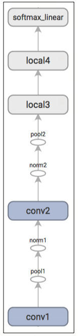
Model Prediction

The prediction part of the model is constructed by the inference() function which adds operations to compute the logits of the predictions. That part of the model is organized as follows:

Layer Name	Description
`conv1`	`tf.nn.conv2d` and `tf.nn.relu` activation.
`pool1`	`tf.nn.max_pool`.
`norm1`	`tf.nn.local_response_normalization`.
`conv2`	`tf.nn.conv2d` and `tf.nn.relu` activation.
`norm2`	`tf.nn.local_response_normalization`.
`pool2`	`tf.nn.max_pool`.
`local3`	fully connected layer with rectified linear activation.
`local4`	fully connected layer with rectified linear activation.
`softmax_linear`	linear transformation to produce logits.

Here is a graph generated from TensorBoard describing the inference operation:

EXERCISE: The output of inference are un-normalized logits. Try editing the network architecture to return normalized predictions using tf.nn.softmax.

The inputs() and inference() functions provide all the components necessary to perform an evaluation of a model. We now shift our focus towards building operations for training a model.

EXERCISE: The model architecture in inference() differs slightly from the CIFAR-10 model specified in cuda-convnet. In particular, the top layers of Alex's original model are locally connected and not fully connected. Try editing the architecture to exactly reproduce the locally connected architecture in the top layer.

Model Training

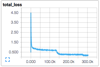
The usual method for training a network to perform N-way classification is multinomial logistic regression, aka. softmax regression. Softmax regression applies a tf.nn.softmax nonlinearity to the output of the network and calculates thetf.nn.sparse_softmax_cross_entropy_with_logits between the normalized predictions and the label index. For regularization, we also apply the usual tf.nn.l2_loss losses to all learned variables. The objective function for the model is the sum of the cross entropy loss and all these weight decay terms, as returned by the loss() function.

We visualize it in TensorBoard with a tf.summary.scalar:

CIFAR-10 Loss

We train the model using standard gradient descent algorithm (see Training for other methods) with a learning rate that tf.train.exponential_decay over time.

CIFAR-10 Learning Rate Decay

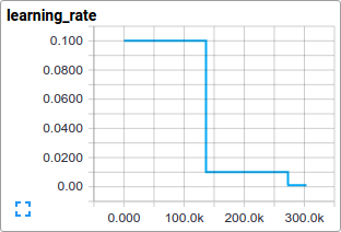
The train() function adds the operations needed to minimize the objective by calculating the gradient and updating the learned variables (see tf.train.GradientDescentOptimizer for details). It returns an operation that executes all the calculations needed to train and update the model for one batch of images.

Launching and Training the Model

We have built the model, let's now launch it and run the training operation with the script cifar10_train.py.

python cifar10_train.py

NOTE: The first time you run any target in the CIFAR-10 tutorial, the CIFAR-10 dataset is automatically downloaded. The data set is ~160MB so you may want to grab a quick cup of coffee for your first run.

You should see the output:

Filling queue with 20000 CIFAR images before starting to train. This will take a few minutes. 2015-11-04 11:45:45.927302: step 0, loss = 4.68 (2.0 examples/sec; 64.221 sec/batch) 2015-11-04 11:45:49.133065: step 10, loss = 4.66 (533.8 examples/sec; 0.240 sec/batch) 2015-11-04 11:45:51.397710: step 20, loss = 4.64 (597.4 examples/sec; 0.214 sec/batch) 2015-11-04 11:45:54.446850: step 30, loss = 4.62 (391.0 examples/sec; 0.327 sec/batch) 2015-11-04 11:45:57.152676: step 40, loss = 4.61 (430.2 examples/sec; 0.298 sec/batch) 2015-11-04 11:46:00.437717: step 50, loss = 4.59 (406.4 examples/sec; 0.315 sec/batch) ...

The script reports the total loss every 10 steps as well as the speed at which the last batch of data was processed. A few comments:

The first batch of data can be inordinately slow (e.g. several minutes) as the preprocessing threads fill up the shuffling queue with 20,000 processed CIFAR images.
The reported loss is the average loss of the most recent batch. Remember that this loss is the sum of the cross entropy and all weight decay terms.
Keep an eye on the processing speed of a batch. The numbers shown above were obtained on a Tesla K40c. If you are running on a CPU, expect slower performance.

EXERCISE: When experimenting, it is sometimes annoying that the first training step can take so long. Try decreasing the number of images that initially fill up the queue. Search for min_fraction_of_examples_in_queue in cifar10_input.py.

cifar10_train.py periodically uses a tf.train.Saver to save all model parameters incheckpoint files but it does not evaluate the model. The checkpoint file will be used by cifar10_eval.py to measure the predictive performance (see Evaluating a Model below).

If you followed the previous steps, then you have now started training a CIFAR-10 model. Congratulations!

The terminal text returned from cifar10_train.py provides minimal insight into how the model is training. We want more insight into the model during training:

Is the loss really decreasing or is that just noise?
Is the model being provided appropriate images?
Are the gradients, activations and weights reasonable?
What is the learning rate currently at?

TensorBoard provides this functionality, displaying data exported periodically from cifar10_train.py via a tf.summary.FileWriter.

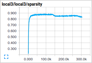
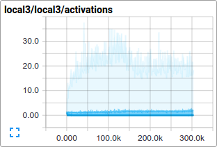
For instance, we can watch how the distribution of activations and degree of sparsity in local3features evolve during training:

Individual loss functions, as well as the total loss, are particularly interesting to track over time. However, the loss exhibits a considerable amount of noise due to the small batch size employed by training. In practice we find it extremely useful to visualize their moving averages in addition to their raw values. See how the scripts use tf.train.ExponentialMovingAverage for this purpose.

Evaluating a Model

Let us now evaluate how well the trained model performs on a hold-out data set. The model is evaluated by the script cifar10_eval.py. It constructs the model with the inference()function and uses all 10,000 images in the evaluation set of CIFAR-10. It calculates the precision at 1: how often the top prediction matches the true label of the image.

To monitor how the model improves during training, the evaluation script runs periodically on the latest checkpoint files created by the cifar10_train.py.

python cifar10_eval.py

Be careful not to run the evaluation and training binary on the same GPU or else you might run out of memory. Consider running the evaluation on a separate GPU if available or suspending the training binary while running the evaluation on the same GPU.

You should see the output:

2015-11-06 08:30:44.391206: precision @ 1 = 0.860 ...

The script merely returns the precision @ 1 periodically -- in this case it returned 86% accuracy. cifar10_eval.py also exports summaries that may be visualized in TensorBoard. These summaries provide additional insight into the model during evaluation.

The training script calculates the tf.train.ExponentialMovingAverage of all learned variables. The evaluation script substitutes all learned model parameters with the moving average version. This substitution boosts model performance at evaluation time.

EXERCISE: Employing averaged parameters may boost predictive performance by about 3% as measured by precision @ 1. Edit cifar10_eval.py to not employ the averaged parameters for the model and verify that the predictive performance drops.

Training a Model Using Multiple GPU Cards

Modern workstations may contain multiple GPUs for scientific computation. TensorFlow can leverage this environment to run the training operation concurrently across multiple cards.

Training a model in a parallel, distributed fashion requires coordinating training processes. For what follows we term model replica to be one copy of a model training on a subset of data.

Naively employing asynchronous updates of model parameters leads to sub-optimal training performance because an individual model replica might be trained on a stale copy of the model parameters. Conversely, employing fully synchronous updates will be as slow as the slowest model replica.

In a workstation with multiple GPU cards, each GPU will have similar speed and contain enough memory to run an entire CIFAR-10 model. Thus, we opt to design our training system in the following manner:

Place an individual model replica on each GPU.
Update model parameters synchronously by waiting for all GPUs to finish processing a batch of data.

Here is a diagram of this model:

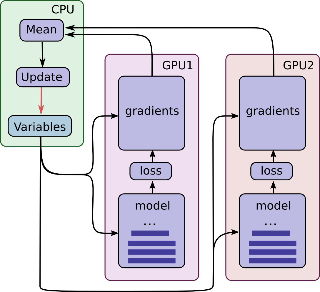
Note that each GPU computes inference as well as the gradients for a unique batch of data. This setup effectively permits dividing up a larger batch of data across the GPUs.

This setup requires that all GPUs share the model parameters. A well-known fact is that transferring data to and from GPUs is quite slow. For this reason, we decide to store and update all model parameters on the CPU (see green box). A fresh set of model parameters is transferred to the GPU when a new batch of data is processed by all GPUs.

The GPUs are synchronized in operation. All gradients are accumulated from the GPUs and averaged (see green box). The model parameters are updated with the gradients averaged across all model replicas.

Placing Variables and Operations on Devices

Placing operations and variables on devices requires some special abstractions.

The first abstraction we require is a function for computing inference and gradients for a single model replica. In the code we term this abstraction a "tower". We must set two attributes for each tower:

A unique name for all operations within a tower. tf.name_scope provides this unique name by prepending a scope. For instance, all operations in the first tower are prepended with tower_0, e.g. tower_0/conv1/Conv2D.
A preferred hardware device to run the operation within a tower. tf.device specifies this. For instance, all operations in the first tower reside within device('/device:GPU:0') scope indicating that they should be run on the first GPU.

All variables are pinned to the CPU and accessed via tf.get_variable in order to share them in a multi-GPU version. See how-to on Sharing Variables.

Launching and Training the Model on Multiple GPU cards

If you have several GPU cards installed on your machine you can use them to train the model faster with the cifar10_multi_gpu_train.py script. This version of the training script parallelizes the model across multiple GPU cards.

python cifar10_multi_gpu_train.py --num_gpus=2

Note that the number of GPU cards used defaults to 1. Additionally, if only 1 GPU is available on your machine, all computations will be placed on it, even if you ask for more.

EXERCISE: The default settings for cifar10_train.py is to run on a batch size of 128. Try running cifar10_multi_gpu_train.py on 2 GPUs with a batch size of 64 and compare the training speed.

Next Steps

If you are now interested in developing and training your own image classification system, we recommend forking this tutorial and replacing components to address your image classification problem.

EXERCISE: Download the Street View House Numbers (SVHN) data set. Fork the CIFAR-10 tutorial and swap in the SVHN as the input data. Try adapting the network architecture to improve predictive performance.

tensorflow随笔-reader(6)