Planar data classification with one hidden layer
Welcome to your week 3 programming assignment. It's time to build your first neural network, which will have a hidden layer. You will see a big difference between this model and the one you implemented using logistic regression.
You will learn how to:
- Implement a 2-class classification neural network with a single hidden layer
- Use units with a non-linear activation function, such as tanh
- Compute the cross entropy loss
- Implement forward and backward propagation
1 - Packages
Let’s first import all the packages that you will need during this assignment.
- numpy is the fundamental package for scientific computing with Python.
- sklearn provides simple and efficient tools for data mining and data analysis.
- matplotlib is a library for plotting graphs in Python.
- testCases provides some test examples to assess the correctness of your functions
- planar_utils provide various useful functions used in this assignment
# Package imports
import numpy as np
import matplotlib.pyplot as plt
from testCases import *
import sklearn
import sklearn.datasets
import sklearn.linear_model
from planar_utils import plot_decision_boundary, sigmoid, load_planar_dataset, load_extra_datasets

%matplotlib inline

np.random.seed(1) # set a seed so that the results are consistent
2 - Dataset
First, let's get the dataset you will work on. The following code will load a "flower" 2-class dataset into variables X and Y.
X, Y = load_planar_dataset()Visualize the dataset using matplotlib. The data looks like a "flower" with some red (label y=0) and some blue (y=1) points. Your goal is to build a model to fit this data.
plt.scatter(X[0, :], X[1, :], c=Y.reshape(X[0,:].shape),   s=40, cmap=plt.cm.Spectral)#此处要squeeze一下,否则可能报错
plt.show()
You have:
- a numpy-array (matrix) X that contains your features (x1, x2)
- a numpy-array (vector) Y that contains your labels (red:0, blue:1).
Lets first get a better sense of what our data is like.
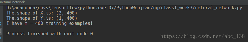
Exercise: How many training examples do you have? In addition, what is the shape of the variables X and Y?
Hint: How do you get the shape of a numpy array? (help)
# 如何得到一个numpy数组的维度

shape_X = np.shape(X)
shape_Y = np.shape(Y)
m = X.shape[1]      #训练集大小


print("The shape of X is: " + str(shape_X))
print("The shape of Y is: " + str(shape_Y))
print("I have m = %d training examples! " % m)
3 - Simple Logistic Regression
Before building a full neural network, lets first see how logistic regression performs on this problem. You can use sklearn's built-in functions to do that. Run the code below to train a logistic regression classifier on the dataset.
# Train the logistic regression classifier
clf = sklearn.linear_model.LogisticRegressionCV();
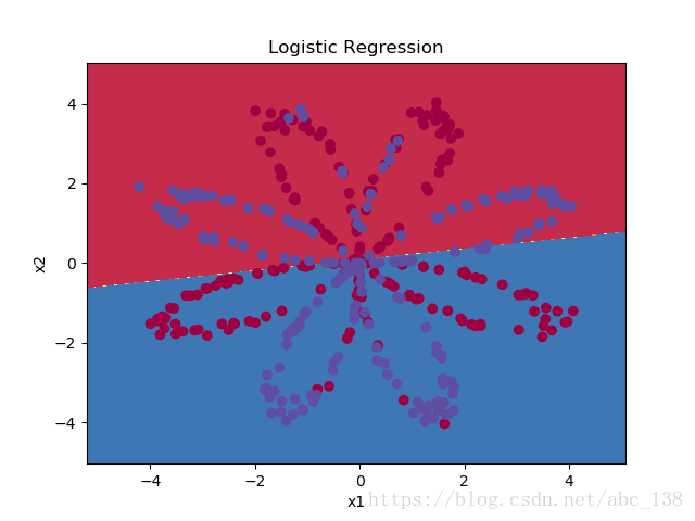
clf.fit(X.T, Y.T);You can now plot the decision boundary of these models. Run the code below.
# Plot the decision boundary for logistic regression
#使用模块函数把分类器画出来,一条直线分为的两个部分。
plot_decision_boundary(lambda x: clf.predict(x), X, Y)
plt.title("Logistic Regression")
plt.show()
# Print accuracy
LR_predictions = clf.predict(X.T)
print ('Accuracy of logistic regression: %d ' % float(
    (np.dot(Y, LR_predictions) + np.dot(1 - Y, 1 - LR_predictions)) / float(Y.size) * 100) +
       '% ' + "(percentage of correctly labelled datapoints)")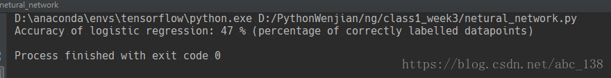
4 - Neural Network model
Logistic regression did not work well on the "flower dataset". You are going to train a Neural Network with a single hidden layer.
Here is our model:
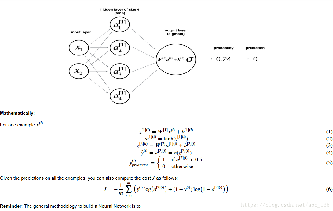
1. Define the neural network structure ( # of input units, # of hidden units, etc).
2. Initialize the model’s parameters
3. Loop:
- Implement forward propagation
- Compute loss
- Implement backward propagation to get the gradients
- Update parameters (gradient descent)
You often build helper functions to compute steps 1-3 and then merge them into one function we call nn_model(). Once you've built nn_model() and learnt the right parameters, you can make predictions on new data.
构建自己的浅层神经网络
该编程作业将实现神经网络的步骤通过一个个的函数来实现,从上到下依次为:
1. 确定各层神经元个数;
2. 初始化参数;
3. 前向传播,求神经网络的输出值;
4. 计算cost;
5. 后向传播,求各参数的偏导数值;
6. 更新各参数值(使用偏导数、学习效率alpha),完成一次迭代;
7. 达到迭代次数,确定神经网络的最终参数;
8. 使用参数修正的神经网络预测样本;
9. 求准确率
4.1 - Defining the neural network structure
Exercise: Define three variables:
- n_x: the size of the input layer
- n_h: the size of the hidden layer (set this to 4)
- n_y: the size of the output layer
Hint: Use shapes of X and Y to find n_x and n_y. Also, hard code the hidden layer size to be 4.
# 定义网络结构
def layer_sizes(X,Y):
"""
参数:
X - 形状输入数据集(输入大小,示例数量)
Y - 形状标签(输出尺寸,示例数量)
返回:
n_x - 输入图层的大小
n_h - 隐藏层的大小
n_y - 输出图层的大小
"""
### START CODE HERE ### (≈ 3 lines of code)
n_x = X.shape[0]
n_h = 4
n_y = Y.shape[0]
### END CODE HERE ###
return (n_x,n_h,n_y)
X_assess,Y_assess = layer_sizes_test_case()
(n_x,n_h,n_y) = layer_sizes(X_assess,Y_assess)
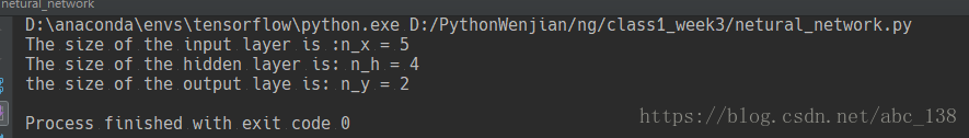
print("The size of the input layer is :n_x = " + str(n_x))
print("The size of the hidden layer is: n_h = " + str(n_h))
print("the size of the output laye is: n_y = " + str(n_y))
4.2 - Initialize the model’s parameters
Exercise: Implement the function initialize_parameters().
Instructions:
- Make sure your parameters’ sizes are right. Refer to the neural network figure above if needed.
- You will initialize the weights matrices with random values.
- Use: np.random.randn(a,b) * 0.01 to randomly initialize a matrix of shape (a,b).
- You will initialize the bias vectors as zeros.
- Use: np.zeros((a,b)) to initialize a matrix of shape (a,b) with zeros.
"""
实现函数initialize_parameters()。
说明:
•确保您的参数尺寸正确。如果需要,请参考上面的神经网络图。
•您将用随机值初始化权重矩阵。 ◾使用:np.random.randn(a,b)* 0.01来随机初始化一个形状矩阵(a,b)。
•您将将偏置向量初始化为零。 ◾使用:np.zeros((a,b))用零初始化形状矩阵(a,b)
"""
# 初始化参数W,b
def initialize_parameters(n_x,n_h,n_y):
"""
输入:
n_x - 输入图层的大小
n_h - 隐藏层的大小
n_y - 输出层的大小
返回:
params - 包含你的参数的python字典:
W1 - 形状的权重矩阵(n_h,n_x)
b1 - 形状的偏向量(n_h,1)
W2 - 形状的权重矩阵(n_y,n_h)
b2 - 形状的偏向量(n_y,1)
"""
np.random.seed(2) #we set up a seed so that your output matches ours although the initialization is random
### START CODE HERE ### (≈ 4 lines of code)
W1 = np.random.randn(n_h,n_x) *0.01
b1 = np.zeros((n_h,1))
W2 = np.random.randn(n_y,n_h) * 0.01
b2 = np.zeros((n_y,1))
### END CODE HERE ###
#assert断言是声明其布尔值必须为真的判定,如果发生异常就说明表达示为假
assert(W1.shape == (n_h,n_x))
assert(b1.shape == (n_h,1))
assert(W2.shape == (n_y,n_h))
assert(b2.shape == (n_y,1))
parameters = {
"W1":W1,
"b1":b1,
"W2":W2,
"b2":b2
}
return parameters
n_x,n_h,n_y = initialize_parameters_test_case()
parameters = initialize_parameters(n_x,n_h,n_y)
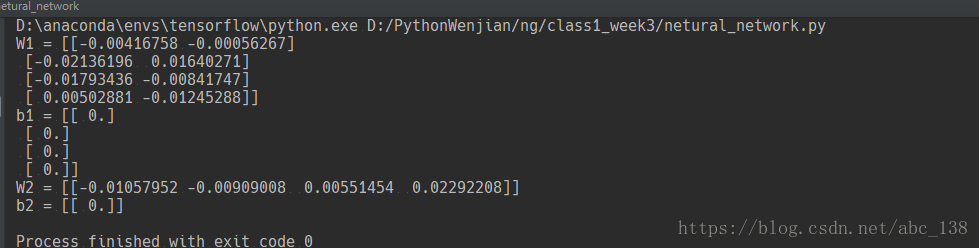
print("W1 = " + str(parameters["W1"]))
print("b1 = " + str(parameters["b1"]))
print("W2 = " + str(parameters["W2"]))
print("b2 = " + str(parameters["b2"]))
4.3 - The Loop
Question: Implement forward_propagation().
Instructions:
- Look above at the mathematical representation of your classifier.
- You can use the function sigmoid(). It is built-in (imported) in the notebook.
- You can use the function np.tanh(). It is part of the numpy library.
- The steps you have to implement are:
1. Retrieve each parameter from the dictionary “parameters” (which is the output of initialize_parameters()) by using parameters[".."].
2. Implement Forward Propagation. Compute Z[1],A[1],Z[2]and (the vector of all your predictions on all the examples in the training set).
- Values needed in the backpropagation are stored in “cache“. The cache will be given as an input to the backpropagation function.
# 前向传播
def forward_propagation(X,parameters):
    """
    输入:
    X - 输入数据的大小(n_x,m)
    参数 - 包含你的参数的python字典(初始化函数的输出)

    返回:
    A2 - 第二次激活的S形输出
    缓存 - 包含“Z1”,“A1”,“Z2”和“A2”的字典
    """
    W1 = parameters["W1"]
    b1 = parameters["b1"]
    W2 = parameters["W2"]
    b2 = parameters["b2"]


    Z1 = np.dot(W1,X) + b1
    A1 = np.tanh(Z1)
    Z2 = np.dot(W2,A1) + b2
    A2 = 1 / (1 + np.exp(-Z2))

    assert (A2.shape == (1,X.shape[1]))
    cache = {
        "Z1":Z1,
        "A1":A1,
        "Z2":Z2,
        "A2":A2
    }
    return A2,cache


X_assess, parameters = forward_propagation_test_case()
A2,cache = forward_propagation(X_assess,parameters)

print(np.mean(cache['Z1']),np.mean(cache['A1']),np.mean(cache['Z2']),np.mean(cache['A2']))

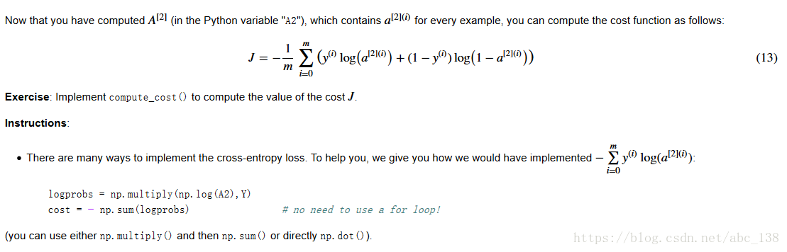
# 计算损失函数
def compute_cost(A2,Y,parameters):
    """
    计算方程(13)中给出的损失函数,

    参数:
    A2 - 第二次激活的S形输出,形状(1,示例数)
    Y - 形状的“真实”标签矢量(1,示例数)
    参数 - 包含您的参数W1,B1,W2和B2的Python字典

    返回:
    成本 - 交叉熵成本给出方程(13)
    """
    m = Y.shape[1]

    logprobs = np.multiply(np.log(A2),Y) + np.multiply(np.log(1-A2),1-Y)       # multiply(a,b)就是个乘法
    cost = -np.sum(logprobs) / m
    cost = np.squeeze(cost)
    assert (isinstance(cost,float))                                           #要判断两个类型是否相同使用 isinstance()

    return cost

A2 ,Y_assess,parameters = compute_cost_test_case()
print("cost = " + str(compute_cost(A2,Y_assess,parameters)))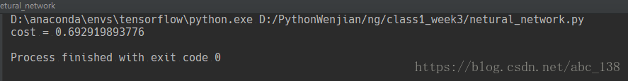
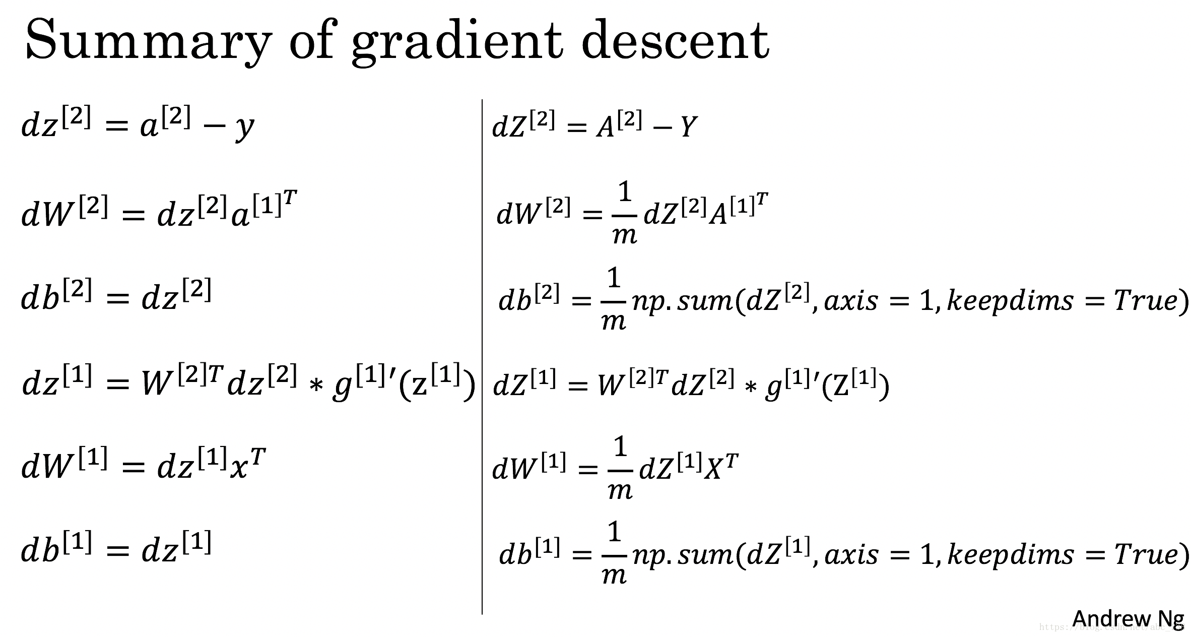
Using the cache computed during forward propagation, you can now implement backward propagation.
Question: Implement the function backward_propagation().
Instructions: Backpropagation is usually the hardest (most mathematical) part in deep learning. To help you, here again is the slide from the lecture on backpropagation. You'll want to use the six equations on the right of this slide, since you are building a vectorized implementation.

# 反向传播
def backward_propagation(parameters,cache,X,Y):
    """
    参数:
    参数 - 包含我们的参数的python字典
    缓存 - 包含“Z1”,“A1”,“Z2”和“A2”的字典。
    X形状的输入数据(2,示例数)
    Y - 形状的“真实”标签矢量(1,示例数)

    返回:
    grads - 包含你的梯度相对于不同参数的python字典
    """
    m = X.shape[1]
    W1 = parameters["W1"]
    W2 = parameters["W2"]
    A1 = cache["A1"]
    A2 = cache["A2"]

    dZ2 = A2 - Y
    dW2 = np.dot(dZ2,A1.T) / m
    db2 = np.sum(dZ2,axis = 1,keepdims= True) /m
    dZ1 = np.multiply(np.dot(W2.T,dZ2),(1-np.power(A1,2)))
    dW1 = np.dot(dZ1,X.T) / m
    db1 = np.sum(dZ1,axis = 1, keepdims= True)

    grads = {
        "dW1":dW1,
        "db1":db1,
        "dW2":dW2,
        "db2":db2
        }
    return grads

parameters,cache,X_assess,Y_assess, = backward_propagation_test_case()
grads = backward_propagation(parameters,cache,X_assess,Y_assess)
print("dW1 = " + str(grads["dW1"]))
print("db1 = " + str(grads["db1"]))
print("dW2 = " + str(grads["dW2"]))
print("db2 = " + str(grads["db2"]))

# 使用dW,db来更新w,b
def update_parameters(parameters,grads,learning_rate = 1.2):
    """
    输入:
    参数 - 包含你的参数的python字典
    grads - 包含你的渐变的python字典

    返回:
    参数 - 包含更新参数的python字典
    """
    W1 = parameters["W1"]
    b1 = parameters["b1"]
    W2 = parameters["W2"]
    b2 = parameters["b2"]

    dW1 = grads["dW1"]
    db1 = grads["db1"]
    dW2 = grads["dW2"]
    db2 = grads["db2"]

    W1 = W1 - learning_rate * dW1
    b1 = b1 - learning_rate * db1
    W2 = W2 - learning_rate * dW2
    b2 = b2 - learning_rate * db2

    parameters = {
        "W1":W1,
        "b1":b1,
        "W2":W2,
        "b2":b2
    }
    return parameters


parameters,grads = update_parameters_test_case()
parameters = update_parameters(parameters,grads)

print("W1 = " + str(parameters["W1"]))
print("b1 = " + str(parameters["b1"]))
print("W2 = " + str(parameters["W2"]))
print("b2 = " + str(parameters["b2"]))
4.4 - Integrate parts 4.1, 4.2 and 4.3 in nn_model()
Question: Build your neural network model in nn_model().
Instructions: The neural network model has to use the previous functions in the right order.
# 把之前写的整合到nn_model中
def nn_model(X,Y,n_h,num_iterations = 10000,print_cost = False):
"""
参数:
X - 形状数据集(2,示例数)
Y - 形状标签(1,示例数)
n_h - 隐藏层的大小
num_iterations - 渐变下降循环中的迭代次数
print_cost - 如果为True,则每1000次迭代打印一次成本
返回:
参数 - 模型学习的参数。然后他们可以用来预测
"""
np.random.seed(3)
n_x = layer_sizes(X,Y)[0]
n_y = layer_sizes(X,Y)[2]
# Initialize parameters, then retrieve W1, b1, W2, b2. Inputs: "n_x, n_h, n_y". Outputs = "W1, b1, W2, b2, parameters".
parameters = initialize_parameters(n_x,n_h,n_y)
W1 = parameters["W1"]
b1 = parameters["b1"]
W2 = parameters["W2"]
b2 = parameters["b2"]
for i in range(0,num_iterations):
# Forward propagation. Inputs: "X, parameters". Outputs: "A2, cache".
A2,cache = forward_propagation(X,parameters)
# Cost function. Inputs: "A2, Y, parameters". Outputs: "cost".
cost = compute_cost(A2,Y,parameters)
# Backpropagation. Inputs: "parameters, cache, X, Y". Outputs: "grads".
grads = backward_propagation(parameters,cache,X,Y)
# Gradient descent parameter update. Inputs: "parameters, grads". Outputs: "parameters".
parameters = update_parameters(parameters,grads,learning_rate = 1.2)
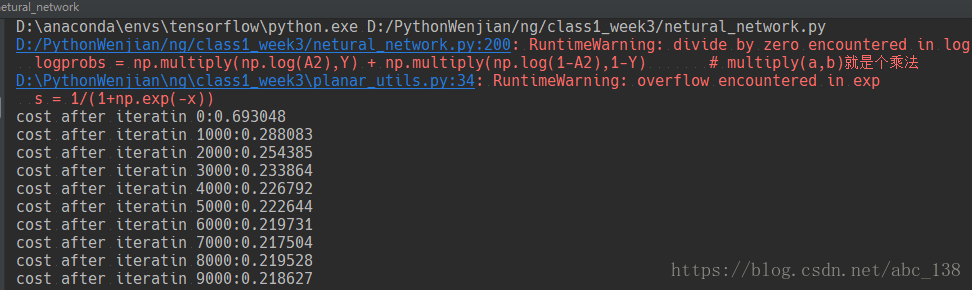
# Print the cost every 1000 iterations
if print_cost and i % 1000 ==0:
print("cost after iteratin %i:%f" % (i,cost))
return parameters
X_assess,Y_assess = nn_model_test_case()
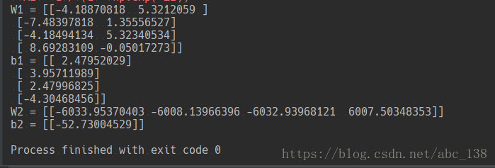
parameters = nn_model(X_assess,Y_assess,4,num_iterations=10000,print_cost = False)
print("W1 = " + str(parameters["W1"]))
print("b1 = " + str(parameters["b1"]))
print("W2 = " + str(parameters["W2"]))
print("b2 = " + str(parameters["b2"]))
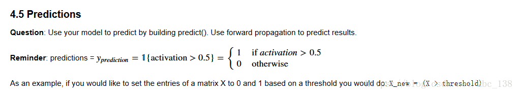
# 预测
def predict(parameters,X):
    """
    参数 - 包含你的参数的python字典
    X - 输入数据的大小(n_x,m)

    返回
    预测 - 我们模型预测的向量(红色:0 /蓝色:1)
    """
    # Computes probabilities using forward propagation, and classifies to 0/1 using 0.5 as the threshold.
    A2 , cache = forward_propagation(X,parameters)
    predictions = (A2 > 0.5)

    return predictions

parameters,X_assess = predict_test_case()
predictions = predict(parameters,X_assess)
print("predictions mean = " + str(np.mean(predictions)))
It is time to run the model and see how it performs on a planar dataset. Run the following code to test your model with a single hidden layer of nh hidden units.
# 我们已经实现了完整的神经网络模型和预测函数,接下来,我们用我们的数据集来训练一下
parameters= nn_model(X,Y,n_h = 4,num_iterations=10000,print_cost=True)
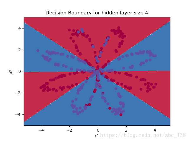
# plot the decision boundary
plot_decision_boundary(lambda x: predict(parameters,x.T),X,Y)
plt.title("Decision Boundary for hidden layer size " + str(4))
plt.show()
predictions = predict(parameters,X)
print("Accuracy: %d " % float((np.dot(Y,predictions.T) + np.dot(1-Y,1-predictions.T))/float(Y.size)*100) + '%')
Accuracy: 90 %Accuracy is really high compared to Logistic Regression. The model has learnt the leaf patterns of the flower! Neural networks are able to learn even highly non-linear decision boundaries, unlike logistic regression.
Now, let's try out several hidden layer sizes.
# 调整隐藏层神经元的数目来观察结果

plt.figure(figsize=(16,32))
hidden_layer_sizes = [1,2,3,4,5,10,20]

for i ,n_h in enumerate(hidden_layer_sizes):
    plt.subplot(5,2,i+1)
    plt.title("Hidden Layer of size %d" % n_h)
    parameters = nn_model(X,Y,n_h,num_iterations=5000)
    plot_decision_boundary(lambda x: predict(parameters,x.T),X,Y)
    # plt.show()
    predictions = predict(parameters, X)
    accuracy = float((np.dot(Y,predictions.T) + np.dot(1-Y,1-predictions.T))/float(Y.size)*100)
    print("Accuracy for {} hidden units: {} %".format(n_h,accuracy))
plt.show()
Accuracy for 1 hidden units: 67.5 %
Accuracy for 2 hidden units: 67.25 %
Accuracy for 3 hidden units: 90.75 %
Accuracy for 4 hidden units: 90.5 %
Accuracy for 5 hidden units: 91.25 %
Accuracy for 10 hidden units: 90.25 %
Accuracy for 20 hidden units: 90.5 %

Interpretation:
- The larger models (with more hidden units) are able to fit the training set better, until eventually the largest models overfit the data.
- The best hidden layer size seems to be around n_h = 5. Indeed, a value around here seems to fits the data well without also incurring noticable overfitting.
- You will also learn later about regularization, which lets you use very large models (such as n_h = 50) without much overfitting.
Optional questions:
Note: Remember to submit the assignment but clicking the blue “Submit Assignment” button at the upper-right.
Some optional/ungraded questions that you can explore if you wish:
- What happens when you change the tanh activation for a sigmoid activation or a ReLU activation?
- Play with the learning_rate. What happens?
- What if we change the dataset? (See part 5 below!)
You’ve learnt to:
- Build a complete neural network with a hidden layer
- Make a good use of a non-linear unit
- Implemented forward propagation and backpropagation, and trained a neural network
- See the impact of varying the hidden layer size, including overfitting.