PS;再看这篇文章前，先要了解什么是判别模型、生成模型。

再看看如下问题，，，

1. GAN对噪声z的分布有要求吗？常用哪些分布？

一般没有特别要求，常用有高斯分布、均匀分布。噪声的维数至少要达到数据流形的内在维数，才能产生足够的diversity，mnist大概是6维，CelebA大概是20维（参考：https://zhuanlan.zhihu.com/p/26528060）

2. GAN的 adversarial 体现在哪里？

G和D的博弈，G需要尽量贴近p_data，D需要识别出真实数据和G生成的数据

3. G和D的loss分别是什么？p_data和p_g的JS divergence和adversarial loss之间存在什么关系？

D的loss 伯努利分布的对数似然函数

G的loss

zero game时，Equation 1
实际训练,Equation 2
不用zero game loss的原因，In practice, equation 1 may not provide sufficient gradient for G to learn well. Early in learning,when G is poor, D can reject samples with high confidence because they are clearly different fromthe training data. In this case, log(1 − D(G(z))) saturates. Rather than training G to minimizelog(1 − D(G(z))) we can train G to maximize log D(G(z)). This objective function results in thesame fixed point of the dynamics of G and D but provides much stronger gradients early in learning.

GAN优化的目标是JSD，是指在D最优的时候，GAN的目标才等价于JSD。

4. 在一轮迭代中，G和D的更新次数哪个多？为了让G学得更好一点，能不能让G多更新？

D更新次数更多，如果G更新太多次会导致diversity不足。

in particular, G must not be trained too much without updating D, in order to avoid “the Helvetica scenario” in which G collapses too many values of z to the same value of x to have enough diversity to model p_data
Optimizing D to completion in the inner loop of training is computationally prohibitive, and on finite datasets would result in overfitting. Instead, we alternate between k steps of optimizing D and one step of optimizing G. This results in D being maintained near its optimal solution, so long as G changes slowly enough.

5. 在GAN中添加batch normalization层有什么作用？

更稳定：

解决随机初始化参数不理想，
防止梯度爆炸，只是降低概率，其他不可控因素还是可能导致梯度爆炸

DCGAN中经验：

Directly applying batchnorm to all layers however, resulted in sample oscillation and model instability. This was avoided by not applying batchnorm to the generator output layer and the discriminator input layer

6. DCGAN对激活函数做了哪些限制？ DCGAN哪些地方使用卷积，哪些地方使用反卷积(fractional-strided卷积)，哪些地方使用全连接？

激活函数：
- G: ReLU, output tanh
- D: leaky rectified activation (GAN mahout), output softmax/sigmoit
卷积应该是D降采样用的，反卷积是G上采样用的
全连接层: 去掉

7. GAN的隐空间的每个维度是否有明确的含义？

原始的GAN应该没有明确含义，它们都交织在一起了，共同决定生成图像的某些属性。
后来的论文，infogan、acgan，对隐空间做disentangle就有了

==================================================

自蒙特利尔大学的Ian Goodfellow等人提出生成式对抗网络（Generative Adversarial Networks，GAN）的概念以来，GAN呈现出井喷式发展。

这篇发布在O’Reilly上的文章中，作者向初学者进行了GAN基础知识答疑，并手把手教给大家如何用GAN创建可以生成手写数字的程序。

本教程由两人完成：Jon Bruner是O’Reilly编辑组的一员，负责管理硬件、互联网、制造和电子学等方面的出版物；Adit Deshpande是加州大学洛杉矶分校计算机科学专业的大二学生。

判别网络

判别器就是一个典型的CNN，它能将二维或三维的像素值矩阵（matrix of pixel values）转化成一个概率。然而作为一个生成器，需要d-维度向量 d-dimensional vector ，并需要将其变为28*28的图像。ReLU和批量标准化（batch normalization）也经常用于稳定每一层的输出。

判别器的结构与TensorFlow的样例CNN分类模型密切相关。它有两层特征为5×5像素特征的卷积层，还有两个全连接层按图像中每个像素计算增加权重的层。

创建了神经网络后，通常需要将权重和偏差初始化，这项任务可以在tf.get_variable中完成。权重在截断正态分布中被初始化，偏差在0处被初始化。

tf.nn.conv2d()是TensorFlow中的标准卷积函数，它包含四个参数：首个参数就是输入图像（input volume）,也就是本示例中的28×28像素的图片；第二个参数是滤波器/权矩阵，最终你也可以改变卷积的“步幅”和“填充”。这两个参数控制着输出图像的尺寸大小。

其实上面这些就是一个普通简单的二进制分类器，如果你不是初次接触CNN，应该对此并不陌生。

定义了判别器之后，我们需要回头看看生成模型。我们将以Tim O’Shea编写的简单生成器代码为基础构建模型的整体结构。

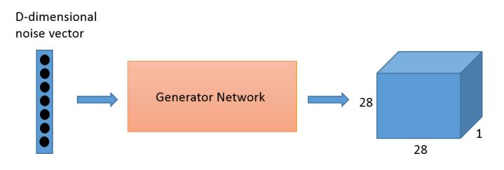
其实你可以把生成器想象成反向卷积神经网络的一种。判别器就是一个典型的CNN，它能将二维或三维的像素值矩阵（matrix of pixel values）转化成一个概率。然而作为一个生成器，需要d-维度向量 d-dimensional vector ，并需要将其变为28*28的图像。ReLU和批量标准化（batch normalization）也经常用于稳定每一层的输出。

在这个神经网络中，我们用了三个卷积层和插值，直到形成28*28像素的图像。

我们在输出层添加了一个tf.sigmoid() 激活函数，它将挤压灰色呈现白色或黑色相，从而产生一个更清晰的图像。

看起来像噪音对吧。现在我们需要训练生成网络中的权重和偏差，将随机数转变为可识别的数字。我们再看看损失函数和优化。

训练GAN

构建和调试GAN就复杂在它有两个损失函数：一个鼓励生成器创造出更好的图像，另一个鼓励判别器区分哪个是真图像，哪个是生成器生成的。

我们同时训练生成器和判别器，当判别器能够很好区分图像来自哪里时，生成器也能更好地调整它的权重和偏差来生成更以假乱真的图像。

所以，让我们首先考虑一下我们需要在网络中得到什么。判别器的目标是正确地将MNIST图像标记为真，而判别器生成的标记为假。我们将计算判别器的两种损失：Dx和1（代表MNIST中的真实图像）的损失，以及Dg与0（代表生成图像）的损失。我们将这个函数在TensorFlow中的tf.nn.sigmoid_cross_entropy_with_logits()函数上运行，计算Dx和0与Dg和1之间的交叉熵损失。

下一步，你需要制定两个优化器，我们一般选择Adam优化算法，它利用了自适应学习速率和动量。我们调用Adam最小函数并且指定我们想更新的变量——也就是我们训练生成器时的生成器权重和偏差，和我们训练判别器时的判别器权重和偏差。

我们为判别器设置了两套不同的训练方案：一种是用真实图像训练判别器，另一种是用生成的“假图像”训练它。有时使用不同的学习速率很有必要，或者单独使用它们来规范学习的其他方面。

收敛GAN是一件棘手的事情，经常需要训练很长时间。可以用TensorBoard追踪训练过程：它可以用图表描绘标量属性（如损失），展示训练中的样本图像，并展示神经网络中的拓扑结构。

现在先给判别器几个简单的原始训练进行迭代，这种方法有助于形成对生成器有用的梯度。

之后我们继续进行主要的训练循环。当训练生成器的时候，我们需要将随机的z向量输入到生成器中，并将其输出传递给判别器（这就是我们早先定义的Dg变量）。生成器的权重和偏差将被改变，主要是为了生成能骗过判别器的图像。

为了训练判别器，我们将给它提供一组来自MNIST数据集中的正面例子，并且再次用生成的图像训练判别器，用它们作为反面例子。

因为训练GAN通常需要很长时间，所以我们建议如果您是第一次使用这个教程，建议先不要运行这个代码块。但你可以先执行下面的代码块，让它生成出一个预先训练模型。

如果你想自己运行这个代码块，请做好长时间等待的准备：在速度相对较快的GPU上运行大概需要3小时，在台式机的CPU上可能耗费10倍时间。

所以，建议你跳过上面直接执行下面的cell。它加载了一个我们在高速GPU机器上训练了10小时的模型，你可以试验下训练过的GAN。

训练不易

众所周知训练GAN很艰难。在没有正确的超参数、网络体系结构和培训流程的情况下，判别器会压制生成器。

一个常见的故障模式是，判别器压制了生成器，肯定地把生成图像定义为假的。当判别器以绝对肯定时，会使生成器无梯度可降。这就是为什么我们建立判别器来产生未缩放的输出，而不是通过一个sigmoid函数将其输出推到0或1。

在另一种常见的故障模式（模式崩溃）中，生成器发现并利用了判别器中的一些弱点，如果它不顾生成器输入z.变量，生成了很多相似图像，你是可以识别出这种模式崩溃的。模式崩溃有时可以通过“强化”鉴别器来修正，例如通过调整其训练速率或重新配置它的层。

先看main.py：

with tf.Session(config=run_config) as sess:
  if FLAGS.dataset == 'mnist':
    dcgan = DCGAN(
        sess,
        input_width=FLAGS.input_width,
        input_height=FLAGS.input_height,
        output_width=FLAGS.output_width,
        output_height=FLAGS.output_height,
        batch_size=FLAGS.batch_size,
        y_dim=10,
        c_dim=1,
        dataset_name=FLAGS.dataset,
        input_fname_pattern=FLAGS.input_fname_pattern,
        is_crop=FLAGS.is_crop,
        checkpoint_dir=FLAGS.checkpoint_dir,
        sample_dir=FLAGS.sample_dir)

因为我们使用DCGAN来生成MNIST数字手写体图像，注意这里的y_dim=10，表示0到9这10个类别，c_dim=1，表示灰度图像。

再看model.py：

def discriminator(self, image, y=None, reuse=False):
  with tf.variable_scope("discriminator") as scope:
    if reuse:
      scope.reuse_variables()
 
    yb = tf.reshape(y, [self.batch_size, 1, 1, self.y_dim])
    x = conv_cond_concat(image, yb)
 
    h0 = lrelu(conv2d(x, self.c_dim + self.y_dim, name='d_h0_conv'))
    h0 = conv_cond_concat(h0, yb)
 
    h1 = lrelu(self.d_bn1(conv2d(h0, self.df_dim + self.y_dim, name='d_h1_conv')))
    h1 = tf.reshape(h1, [self.batch_size, -1])      
    h1 = tf.concat_v2([h1, y], 1)
       
    h2 = lrelu(self.d_bn2(linear(h1, self.dfc_dim, 'd_h2_lin')))
    h2 = tf.concat_v2([h2, y], 1)
 
    h3 = linear(h2, 1, 'd_h3_lin')
        
    return tf.nn.sigmoid(h3), h3

这里batch_size=64，image的维度为[64 28 28 1]，y的维度是[64 10]，yb的维度[64 1 1 10]，x将image和yb连接起来，这相当于是使用了Conditional GAN，为图像提供标签作为条件信息，于是x的维度是[64 28 28 11]，将x输入到卷积层conv2d，conv2d的代码如下：

def conv2d(input_, output_dim, 
       k_h=5, k_w=5, d_h=2, d_w=2, stddev=0.02,
       name="conv2d"):
  with tf.variable_scope(name):
    w = tf.get_variable('w', [k_h, k_w, input_.get_shape()[-1], output_dim],
              initializer=tf.truncated_normal_initializer(stddev=stddev))
    conv = tf.nn.conv2d(input_, w, strides=[1, d_h, d_w, 1], padding='SAME')
 
    biases = tf.get_variable('biases', [output_dim], initializer=tf.constant_initializer(0.0))
    conv = tf.reshape(tf.nn.bias_add(conv, biases), conv.get_shape())
 
    return conv

卷积核的大小为5*5，stride为[1 2 2 1]，通过2的卷积步长可以替代pooling进行降维，padding=‘SAME’，则卷积的输出维度为[64 14 14 11]。然后使用batch normalization及leaky ReLU的激活层，输出与yb再进行concat，得到h0，维度为[64 14 14 21]。同理，h1的维度为[64 7*7*74+10]，h2的维度为[64 1024+10]，然后连接一个线性输出，得到h3，维度为[64 1]，由于我们希望判别器的输出代表概率，所以最终使用一个sigmoid的激活。

def generator(self, z, y=None):
  with tf.variable_scope("generator") as scope:
      
    s_h, s_w = self.output_height, self.output_width
    s_h2, s_h4 = int(s_h/2), int(s_h/4)
    s_w2, s_w4 = int(s_w/2), int(s_w/4)
 
    # yb = tf.expand_dims(tf.expand_dims(y, 1),2)
    yb = tf.reshape(y, [self.batch_size, 1, 1, self.y_dim])
    z = tf.concat_v2([z, y], 1)
 
    h0 = tf.nn.relu(
        self.g_bn0(linear(z, self.gfc_dim, 'g_h0_lin')))
    h0 = tf.concat_v2([h0, y], 1)
 
    h1 = tf.nn.relu(self.g_bn1(
        linear(h0, self.gf_dim*2*s_h4*s_w4, 'g_h1_lin')))
    h1 = tf.reshape(h1, [self.batch_size, s_h4, s_w4, self.gf_dim * 2])
 
    h1 = conv_cond_concat(h1, yb)
 
    h2 = tf.nn.relu(self.g_bn2(deconv2d(h1,
        [self.batch_size, s_h2, s_w2, self.gf_dim * 2], name='g_h2')))
    h2 = conv_cond_concat(h2, yb)
 
    return tf.nn.sigmoid(
        deconv2d(h2, [self.batch_size, s_h, s_w, self.c_dim], name='g_h3'))

output_height和output_width为28，因此s_h和s_w为28，s_h2和s_w2为14，s_h4和s_w4为7。在这里z为平均分布的随机分布数，维度为[64 100]，y的维度为[64 10]，yb的维度是[64 1 1 10]，z与y进行一个concat得到[64 110]的tensor，输入到一个线性层，输出维度是[64 1024]，再经过batch normalization以及ReLU激活，并与y进行concat，输出h0的维度是[64 1034]，同样的再经过一个线性层输出维度为[64 128*7*7]，再进行reshape并与yb进行concat，得到h1，维度为[64 7 7 138]，然后输入到一个deconv2d，做一个反卷积，也就是文中说的fractional strided convolutions，再经过batch normalization以及ReLU激活，并与yb进行concat，输出h2的维度是[64 14 14 138]，最后再输入到deconv2d层以及sigmoid激活，得到生成器的输出，维度为[64 28 28 1]。

生成器以及判别器的输出：

self.G = self.generator(self.z, self.y)
self.D, self.D_logits = \
    self.discriminator(inputs, self.y, reuse=False)
 
self.D_, self.D_logits_ = \
    self.discriminator(self.G, self.y, reuse=True)

其中D表示真实数据的判别器输出，D_表示生成数据的判别器输出。

再看损失函数：

self.d_loss_real = tf.reduce_mean(
  tf.nn.sigmoid_cross_entropy_with_logits(
    logits=self.D_logits, targets=tf.ones_like(self.D)))
self.d_loss_fake = tf.reduce_mean(
  tf.nn.sigmoid_cross_entropy_with_logits(
    logits=self.D_logits_, targets=tf.zeros_like(self.D_)))
self.g_loss = tf.reduce_mean(
  tf.nn.sigmoid_cross_entropy_with_logits(
    logits=self.D_logits_, targets=tf.ones_like(self.D_)))

即对于真实数据，判别器的损失函数d_loss_real为判别器输出与1的交叉熵，而对于生成数据，判别器的损失函数d_loss_fake为输出与0的交叉熵，因此判别器的损失函数d_loss=d_loss_real+d_loss_fake；生成器的损失函数是g_loss判别器对于生成数据的输出与1的交叉熵。
优化器：

d_optim = tf.train.AdamOptimizer(config.learning_rate, beta1=config.beta1) \
          .minimize(self.d_loss, var_list=self.d_vars)
g_optim = tf.train.AdamOptimizer(config.learning_rate, beta1=config.beta1) \
          .minimize(self.g_loss, var_list=self.g_vars)

训练阶段：

for epoch in xrange(config.epoch):
  batch_idxs = min(len(data_X), config.train_size) // config.batch_size
      
  for idx in xrange(0, batch_idxs):
        
    batch_images = data_X[idx*config.batch_size:(idx+1)*config.batch_size]
    batch_labels = data_y[idx*config.batch_size:(idx+1)*config.batch_size]
 
    batch_images = np.array(batch).astype(np.float32)[:, :, :, None]
 
    batch_z = np.random.uniform(-1, 1, [config.batch_size, self.z_dim]) \
          .astype(np.float32)
 
    # Update D network
    _, summary_str = self.sess.run([d_optim, self.d_sum],
      feed_dict={ 
        self.inputs: batch_images,
        self.z: batch_z,
        self.y:batch_labels,
      })
    self.writer.add_summary(summary_str, counter)
 
    # Update G network
    _, summary_str = self.sess.run([g_optim, self.g_sum],
      feed_dict={
        self.z: batch_z, 
        self.y:batch_labels,
      })
    self.writer.add_summary(summary_str, counter)
 
    # Run g_optim twice to make sure that d_loss does not go to zero (different from paper)
    _, summary_str = self.sess.run([g_optim, self.g_sum],
      feed_dict={ self.z: batch_z, self.y:batch_labels })
    self.writer.add_summary(summary_str, counter)
        
    errD_fake = self.d_loss_fake.eval({
        self.z: batch_z, 
        self.y:batch_labels
    })
    errD_real = self.d_loss_real.eval({
        self.inputs: batch_images,
        self.y:batch_labels
    })
    errG = self.g_loss.eval({
        self.z: batch_z,
        self.y: batch_labels
    })
     
    counter += 1

与论文中不同的是，这里在一个batch中，更新两次生成器，更新一次判别器。

How to Train a GAN? Tips and tricks to make GANs work

1. Normalize the inputs

normalize the images between -1 and 1
Tanh as the last layer of the generator output

2: A modified loss function

In GAN papers, the loss function to optimize G is min (log 1-D), but in practice folks practically use max log D

because the first formulation has vanishing gradients early on
Goodfellow et. al (2014)

In practice, works well:

Flip labels when training generator: real = fake, fake = real

3: Use a spherical Z

Dont sample from a Uniform distribution

Sample from a gaussian distribution

When doing interpolations, do the interpolation via a great circle, rather than a straight line from point A to point B
Tom White's Sampling Generative Networks ref code https://github.com/dribnet/plat has more details

4: BatchNorm

Construct different mini-batches for real and fake, i.e. each mini-batch needs to contain only all real images or all generated images.
when batchnorm is not an option use instance normalization (for each sample, subtract mean and divide by standard deviation).

5: Avoid Sparse Gradients: ReLU, MaxPool

the stability of the GAN game suffers if you have sparse gradients
LeakyReLU = good (in both G and D)
For Downsampling, use: Average Pooling, Conv2d + stride
For Upsampling, use: PixelShuffle, ConvTranspose2d + stride
- PixelShuffle: https://arxiv.org/abs/1609.05158

6: Use Soft and Noisy Labels

Label Smoothing, i.e. if you have two target labels: Real=1 and Fake=0, then for each incoming sample, if it is real, then replace the label with a random number between 0.7 and 1.2, and if it is a fake sample, replace it with 0.0 and 0.3 (for example).
- Salimans et. al. 2016
make the labels the noisy for the discriminator: occasionally flip the labels when training the discriminator

7: DCGAN / Hybrid Models

Use DCGAN when you can. It works!
if you cant use DCGANs and no model is stable, use a hybrid model : KL + GAN or VAE + GAN

8: Use stability tricks from RL

Experience Replay
- Keep a replay buffer of past generations and occassionally show them
- Keep checkpoints from the past of G and D and occassionaly swap them out for a few iterations
All stability tricks that work for deep deterministic policy gradients
See Pfau & Vinyals (2016)

9: Use the ADAM Optimizer

optim.Adam rules!
- See Radford et. al. 2015
Use SGD for discriminator and ADAM for generator

10: Track failures early

D loss goes to 0: failure mode
check norms of gradients: if they are over 100 things are screwing up
when things are working, D loss has low variance and goes down over time vs having huge variance and spiking
if loss of generator steadily decreases, then it's fooling D with garbage (says martin)

11: Dont balance loss via statistics (unless you have a good reason to)

Dont try to find a (number of G / number of D) schedule to uncollapse training
It's hard and we've all tried it.
If you do try it, have a principled approach to it, rather than intuition

For example

while lossD > A:
train D
while lossG > B:
train G

12: If you have labels, use them

if you have labels available, training the discriminator to also classify the samples: auxillary GANs

13: Add noise to inputs, decay over time

Add some artificial noise to inputs to D (Arjovsky et. al., Huszar, 2016)
- http://www.inference.vc/instance-noise-a-trick-for-stabilising-gan-training/
- https://openreview.net/forum?id=Hk4_qw5xe
adding gaussian noise to every layer of generator (Zhao et. al. EBGAN)
- Improved GANs: OpenAI code also has it (commented out)

14: [notsure] Train discriminator more (sometimes)

especially when you have noise
hard to find a schedule of number of D iterations vs G iterations

15: [notsure] Batch Discrimination

Mixed results

16: Discrete variables in Conditional GANs

Use an Embedding layer
Add as additional channels to images
Keep embedding dimensionality low and upsample to match image channel size

17: Use Dropouts in G in both train and test phase

Provide noise in the form of dropout (50%).
Apply on several layers of our generator at both training and test time
https://arxiv.org/pdf/1611.07004v1.pdf

reference:

https://github.com/soumith/ganhacks

https://zhuanlan.zhihu.com/p/27440393

GAN 生成对抗网络与 DCGAN 深度卷积生成对抗网络

PS;再看这篇文章前，先要了解什么是判别模型、生成模型。

1. GAN对噪声z的分布有要求吗？常用哪些分布？

2. GAN的 adversarial 体现在哪里？

3. G和D的loss分别是什么？p_data和p_g的JS divergence和adversarial loss之间存在什么关系？

4. 在一轮迭代中，G和D的更新次数哪个多？为了让G学得更好一点，能不能让G多更新？

5. 在GAN中添加batch normalization层有什么作用？

6. DCGAN对激活函数做了哪些限制？ DCGAN哪些地方使用卷积，哪些地方使用反卷积(fractional-strided卷积)，哪些地方使用全连接？

7. GAN的隐空间的每个维度是否有明确的含义？

判别网络

训练GAN

训练不易

How to Train a GAN? Tips and tricks to make GANs work

1. Normalize the inputs

2: A modified loss function

3: Use a spherical Z

4: BatchNorm

5: Avoid Sparse Gradients: ReLU, MaxPool

6: Use Soft and Noisy Labels

7: DCGAN / Hybrid Models

8: Use stability tricks from RL

9: Use the ADAM Optimizer

10: Track failures early

11: Dont balance loss via statistics (unless you have a good reason to)

12: If you have labels, use them

13: Add noise to inputs, decay over time

14: [notsure] Train discriminator more (sometimes)

15: [notsure] Batch Discrimination

16: Discrete variables in Conditional GANs

17: Use Dropouts in G in both train and test phase

猜你喜欢

GAN 生成对抗网络 与 DCGAN 深度卷积生成对抗网络

PS;再看这篇文章前，先要了解什么是判别模型、生成模型。

1. GAN对噪声z的分布有要求吗？常用哪些分布？

2. GAN的 adversarial 体现在哪里？

3. G和D的loss分别是什么？p_data和p_g的JS divergence和adversarial loss之间存在什么关系？

4. 在一轮迭代中，G和D的更新次数哪个多？为了让G学得更好一点，能不能让G多更新？

5. 在GAN中添加batch normalization层有什么作用？

6. DCGAN对激活函数做了哪些限制？ DCGAN哪些地方使用卷积，哪些地方使用反卷积(fractional-strided卷积)，哪些地方使用全连接？

7. GAN的隐空间的每个维度是否有明确的含义？

判别网络

训练GAN

训练不易

How to Train a GAN? Tips and tricks to make GANs work

1. Normalize the inputs

2: A modified loss function

3: Use a spherical Z

4: BatchNorm

5: Avoid Sparse Gradients: ReLU, MaxPool

6: Use Soft and Noisy Labels

7: DCGAN / Hybrid Models

8: Use stability tricks from RL

9: Use the ADAM Optimizer

10: Track failures early

11: Dont balance loss via statistics (unless you have a good reason to)

12: If you have labels, use them

13: Add noise to inputs, decay over time

14: [notsure] Train discriminator more (sometimes)

15: [notsure] Batch Discrimination

16: Discrete variables in Conditional GANs

17: Use Dropouts in G in both train and test phase

猜你喜欢

GAN 生成对抗网络与 DCGAN 深度卷积生成对抗网络