【OpenCV】轮廓检测

轮廓检测的作用：
1.可以检测图图像或者视频中物体的轮廓
2.计算多边形边界，形状逼近和计算感兴趣区域

先看一个较为简单的轮廓检测：

import cv2
import numpy as np
# 创建一个200*200的黑色空白图像
img = np.zeros((200, 200), dtype=np.uint8)
# 利用numpy数组在切片上赋值的功能放置一个白色方块
img[50:150, 50:150] = 255

# 对图像进行二值化操作
# threshold(src, thresh, maxval, type, dst=None)
# src是输入数组，thresh是阈值的具体值，maxval是type取THRESH_BINARY或者THRESH_BINARY_INV时的最大值
# type有5种类型,这里取0： THRESH_BINARY ，当前点值大于阈值时，取maxval，也就是前一个参数，否则设为0
# 该函数第一个返回值是阈值的值，第二个是阈值化后的图像
ret, thresh = cv2.threshold(img, 127, 255, 0)

# findContours()有三个参数：输入图像，层次类型和轮廓逼近方法
# 该函数会修改原图像，建议使用img.copy()作为输入
# 由函数返回的层次树很重要，cv2.RETR_TREE会得到图像中轮廓的整体层次结构，以此来建立轮廓之间的‘关系’。
# 如果只想得到最外面的轮廓，可以使用cv2.RETE_EXTERNAL。这样可以消除轮廓中其他的轮廓，也就是最大的集合
# 该函数有三个返回值：修改后的图像，图像的轮廓，它们的层次
image, contours, hierarchy = cv2.findContours(thresh, cv2.RETR_TREE, cv2.CHAIN_APPROX_SIMPLE)

color = cv2.cvtColor(img, cv2.COLOR_GRAY2BGR)
img = cv2.drawContours(color, contours, -1, (0, 255, 0), 2)
cv2.imshow("contours", color)
cv2.waitKey()
cv2.destroyAllWindows()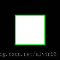

上面是找到一个正方形的轮廓，下面看如何找到不规则的多边形轮廓：

import cv2
import numpy as np

# pyrDown():brief Blurs an image and downsamples it.
# 将图像高斯平滑，然后进行降采样
img = cv2.pyrDown(cv2.imread("hammer.jpg", cv2.IMREAD_UNCHANGED))
# 依然是二值化操作
ret, thresh = cv2.threshold(cv2.cvtColor(img.copy(), cv2.COLOR_BGR2GRAY), 127, 255, cv2.THRESH_BINARY)
# 计算图像的轮廓
image, contours, hier = cv2.findContours(thresh, cv2.RETR_EXTERNAL, cv2.CHAIN_APPROX_SIMPLE)

for c in contours:
    # find bounding box coordinates
    # 先计算出一个简单的边界狂，也就是一个矩形啦
    # 就是将轮廓信息转换为(x,y)坐标，并加上矩形的高度和宽度
    x, y, w, h = cv2.boundingRect(c)
    # 画出该矩形
    cv2.rectangle(img, (x, y), (x + w, y + h), (0, 255, 0), 2)

    # find minimum area
    # 然后计算包围目标的最小矩形区域
    # 这里先计算出最小矩形区域，然后计算区域的顶点，此时顶点坐标是浮点型，但是像素坐标是整数
    # 需要将浮点型转换成矩形
    rect = cv2.minAreaRect(c)
    box = cv2.boxPoints(rect)
    box = np.int0(box)
    # draw contours
    # 画出最小矩形
    # drawContours()也会修改源图像
    # 第二个参数保存轮廓的数组，也就是保存着很多轮廓
    # 第三个参数是要绘制的轮廓数组的索引：-1是绘制所有的轮廓，否则只绘制[box]中指定的轮廓
    # 颜色和thickness(密度,就是粗细)放在最后两个参数
    cv2.drawContours(img, [box], 0, (0, 0, 255), 3)

    # calculate center and radius of minimum enclosing circle
    # 最后检查的边界轮廓为最小闭圆
    # minEnclosingCircle()会返回一个二元数组，第一个是圆心坐标组成的元祖，第二个元素是元的半径
    (x, y), radius = cv2.minEnclosingCircle(c)
    # cast to integers
    center = (int(x), int(y))
    radius = int(radius)
    # draw the circle
    img = cv2.circle(img, center, radius, (255, 0, 0), 3)

# 绘制轮廓
cv2.drawContours(img, contours, -1, (255, 0, 0), 1)
cv2.imshow("contours", img)

cv2.waitKey()
cv2.destroyAllWindows()

凸轮廓与Douglas-Peucker算法

import cv2
import numpy as np

img = cv2.pyrDown(cv2.imread("hammer.jpg", cv2.IMREAD_UNCHANGED))

ret, thresh = cv2.threshold(cv2.cvtColor(img.copy(), cv2.COLOR_BGR2GRAY), 127, 255, cv2.THRESH_BINARY)
# 创建与源图像一样大小的矩阵
black = cv2.cvtColor(np.zeros((img.shape[1], img.shape[0]), dtype=np.uint8), cv2.COLOR_GRAY2BGR)

image, contours, hier = cv2.findContours(thresh, cv2.RETR_EXTERNAL, cv2.CHAIN_APPROX_SIMPLE)

for cnt in contours:
    # 得到轮廓的周长作为参考
    epsilon = 0.01 * cv2.arcLength(cnt,True)
    # approxPolyDP()用来计算近似的多边形框。有三个参数
    # cnt为轮廓，epsilon为ε——表示源轮廓与近似多边形的最大差值，越小越接近
    # 第三个是布尔标记，用来表示这个多边形是否闭合
    approx = cv2.approxPolyDP(cnt,epsilon,True)
    # convexHull()可以从轮廓获取凸形状
    hull = cv2.convexHull(cnt)
    # 源图像轮廓-绿色
    cv2.drawContours(black, [cnt], -1, (0, 255, 0), 2)
    # 近似多边形-蓝色
    cv2.drawContours(black, [approx], -1, (255, 0, 0), 2)
    # 凸包-红色
    cv2.drawContours(black, [hull], -1, (0, 0, 255), 2)

cv2.imshow("hull", black)
cv2.waitKey()
cv2.destroyAllWindows()

本来也有疑问，有了一个精确的轮廓，为什么还需要一个近似的多边形？
书中给出答案，近似多边形是由一组直线构成，这样可以便于后续的操作和处理。
想来也是，直线构成的区域总是比无限个曲率的曲线构成的区域方便处理。

直线和圆检测

直线检测可以通过HoughLinesP函数完成，HoughLinesP是标准Hough变换经过优化，使用概率Hough变换。

import cv2
import numpy as np

img = cv2.imread('lines.jpg')
gray = cv2.cvtColor(img,cv2.COLOR_BGR2GRAY)
edges = cv2.Canny(gray,50,120)
# 最小直线长度，小于该长度会被消除
minLineLength = 20
# 最大线段间隙，一条直线的间隙长度大于这个值会被认为是两条直线
maxLineGap = 5
# HoughLinesP()会接受一个由Canny边缘检测滤波器处理过的单通道二值图像
# 不一定需要Canny滤波器，但是输入是去噪且只有边缘的图像，效果会很好
# 第一个参数是输入图像
# 第二、第三个参数是线段的几何表示rho和theta，一般取1和np.pi/180
# 第四个参数是阈值，低于该阈值的直线会被忽略
# 第五第六已经解释
lines = cv2.HoughLinesP(edges,1,np.pi/180,20,minLineLength,maxLineGap)
for x1,y1,x2,y2 in lines[0]:
    cv2.line(img,(x1,y1),(x2,y2),(0,255,0),2)

cv2.imshow("edges", edges)
cv2.imshow("lines", img)
cv2.waitKey()
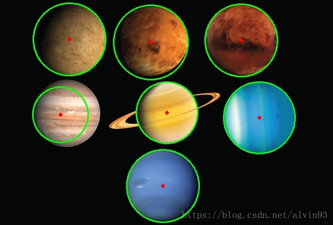
cv2.destroyAllWindows()

圆检测可以通过HoughCircles函数检测。

import cv2
import numpy as np

planets = cv2.imread('planet_glow.jpg')
gray_img = cv2.cvtColor(planets, cv2.COLOR_BGR2GRAY)
img = cv2.medianBlur(gray_img, 5)
cimg = cv2.cvtColor(img, cv2.COLOR_GRAY2BGR)

# 与直线检测类似，需要圆心距的最小距离和圆的最小以及最大半径
circles = cv2.HoughCircles(img,cv2.HOUGH_GRADIENT,1,120,param1=100,param2=30,minRadius=0,maxRadius=0)

circles = np.uint16(np.around(circles))

for i in circles[0,:]:
    # draw the outer circle
    cv2.circle(planets,(i[0],i[1]),i[2],(0,255,0),2)
    # draw the center of the circle
    cv2.circle(planets,(i[0],i[1]),2,(0,0,255),3)

cv2.imwrite("planets_circles.jpg", planets)
cv2.imshow("HoughCirlces", planets)
cv2.waitKey()
cv2.destroyAllWindows()

有一个问题，该方法检测出来的第二行的第一个星球的圆检测与书中不一样。