图灵程序丛书 —《数据科学入门》— Ch4-Ch7 线性代数、统计学、概率、假设与推断

Ch4-Ch7 线性代数、统计学、概率、假设与推断

此系列记录《数据科学入门》学习笔记

Ch 4 线性代数

4.1 向量

# 向量加减法
def vector_add(v, m):
    return [v_i + w_i for v_i, w_i in zip(v, w)]


def vector_subtract(v, m):
    return [v_i - w_i for v_i, w_i in zip(v, w)]

# 一系列向量的加法
def vector_sum(vectors):
    result = vectors[0]
    for vector in vectors[1:]:
        result = vector_add(result, vector)
    return result

def vector_sum1(vectors):
    return reduce(vector_add, vectors)

vector_sum = patial(reduce, vector_add)

# 标量乘以向量
def scalar_multiply(c, v):
    return [c * v_i for v_i in v]

# 计算一系列长度相同的向量的均值
def vector_meam(vectors):
    n = len(vectors)
    return scalar_multiply(1/n, vector_sum(vectors))

# 两个向量的点乘
def dot(v, w):
    return sum(v_i * w_i for v_i, w_i in zip(v, w))

# 计算向量的平方
def sum_of_squares(v):
    return dot(v, v)

# 计算向量的长度、距离
import math
def magnitude(v):
    return math.sqrt(sum_of_squares(v))

def squared_distance(v, w):
    return sum_of_squares(vector_subtract(v, w))

def distance(v, w):
    return math.sqrt(squared_distance(v, w))

def distance(v, w):
    return magnitude(vector_substract(v, w))

4.2 矩阵

# 求维数
def shape(a):
    num_rows = len(a)
    num_cols = len(a[0]) if a else 0
    return num_rows, num_cols

# 返回矩阵的某一行或者某一列
def get_row(a, i):
    return a[i]

def get_col(a, j):
    return a[:,j]

def get_col(a, j):
    return [a_i[j] for a_i in a]

# 根据形状和用来生成元素的函数来创建矩阵
def make_matrix(num_rows, num_cols, entry_fn):
    return [[entry_fn(i, j) for j in range(num_cols)] for i in range(num_rows)]

def is_diagonal(i, j):
    return 1 if i == j else 0

identify_matrix = make_matrix(5, 5, is_diagonal)
identify_matrix
#[[1, 0, 0, 0, 0],
# [0, 1, 0, 0, 0],
# [0, 0, 1, 0, 0],
# [0, 0, 0, 1, 0],
# [0, 0, 0, 0, 1]]

Ch 5 统计学

5.1 描述单个数据集

num_friends = [100, 9, 1, 4, 25, 63, 5, 16, 5, 9, 5, 25, 2, 15, 26, 2, 6, 4, 15, 16, 4, 26, 22, 13, 16, 45,
               23, 8, 9, 15, 6, 12, 5, 85, 12, 14, 2, 17, 5, 13, 42, 51, 5, 4, 26, 2, 4, 9, 5, 12, 6, 19, 
               14, 3, 5, 4, 15, 62, 15, 21, 16, 12, 3, 26, 4, 5, 41, 18, 85, 6, 8, 8, 11, 92, 12, 21, 36, 8]


from collections import Counter
import matplotlib.pyplot as plt
from pylab import *  

friend_counts = Counter(num_friends)
xs = range(max(num_friends))
ys = [friend_counts[x] for x in xs]
plt.bar(xs, ys);
plt.axis([0, 101, 0, 10])
mpl.rcParams['font.sans-serif'] = ['SimHei'] 
plt.title('朋友的数量')
plt.xlabel('朋友个数')
plt.ylabel('人数')
plt.show()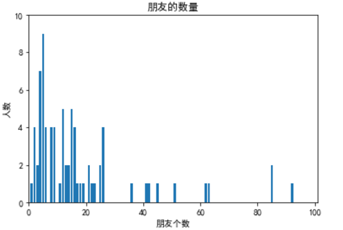

print(len(num_friends))    # 78
print(max(num_friends))    # 100
print(min(num_friends))    # 1
print(sum(num_friends))    # 1441
print(mean(num_friends))   # 18.4743589
print(median(num_friends)) # 12.0


print(sorted(num_friends)[0])    # 1
print(sorted(num_friends)[1])    # 2
print(sorted(num_friends)[-1])   # 100
print(sorted(num_friends)[-2])   # 92

5.1.1 中心倾向

def mean1(x):
    return sum(x) / len(x)
mean1(num_friends)  # 18.4743589

def median1(v):
    n = len(v)
    sortedv = sorted(v)
    if n % 2 == 1:
        return sortedv[n//2 + 1]
    else:
        return (sortedv[n//2] + sortedv[n//2+1])*0.5
median1(num_friends)   # 12.0

def quantile1(x, p):
    p_index = int(p * len(x))
    return sorted(x)[p_index]

print(quantile1(num_friends, 0) == min(num_friends))    # True
print(quantile1(num_friends, 0.1))                      # 4
print(quantile1(num_friends, 0.99) == max(num_friends)) # Ture

def interquantile_range(x):
    return quantile1(x, 0.75) - quantile1(x, 0.25)
interquantile_range(num_friends)   # 16

# 众数
def mode1(x):
    counts = Counter(x)
    max_count = max(counts.values())
    return [x_i for x_i, count in counts.items() if count == max_count]
mode1(num_friends)   # [5]

5.1.2 离散值

def range1(x):
    return max(x) - min(x)
range1(num_friends)   # 99

def de_mean(x):
    x_bar = mean(x)
    return [x_i - x_bar for x_i in x]

def variance(x):
    n = len(x)
    deviantions = de_mean(x)
    return sum_of_squares(deviantions) / (n - 1)

variance(num_friends)   #450.99284

def standard_deviation(x):
    return sqrt(variance(x))
standard_deviation(num_friends)   # 21.35398

5.2 相关

def covariance(x, y):
    n = len(x)
    return dot(de_mean(x), de_mean(y)) / (n - 1)
covariance(num_friends, randn(len(num_friends)))   # -3.47864

def correlation(x, y):
    stdev_x = standard_deviation(x)
    stdev_y = standard_deviation(y)
    if stdev_x > 0 and stdev_y > 0:
        return covariance(x, y) / stdev_x / stdev_y
    else:
        return 0
correlation(num_friends, randn(len(num_friends)))   # 0.051299678

5.3 辛普森悖论

辛普森悖论是指分析数据时可能会发生的意外。具体而言，如果忽略了混杂变量，相关系数会有误导性。

如果没有这200给数据科学家的受教育程度数据，就会直接得到西海岸的数据科学家天生更有社交能力的结论。

<table>
  <tr>
    <th width=33.33%, bgcolor = lightblue> 海岸</th>
    <th width=33.33%, bgcolor = lightblue> 成员数</th>
    <th width=33.33%, bgcolor = lightblue> 平均朋友数</th>
  </tr>
  <tr>
    <td bgcolor=lightgreen> 西海岸 </td>
    <td> 101  </td>
    <td> 8.2  </td>
  </tr>
  <tr>
    <td bgcolor=lightgreen> 东海岸 </td>
    <td> 103 </td>
    <td> 6.5 </td>
  <tr>
</table>

<table>
  <tr>
    <th width=25%, bgcolor = lightblue> 海岸</th>
    <th width=25%, bgcolor = lightblue> 学位</th>
    <th width=25%, bgcolor = lightblue> 成员数</th>
    <th width=25%, bgcolor = lightblue> 平均朋友数</th>
  </tr>
  <tr>
    <td bgcolor=lightgrey> 西海岸 </td>
    <td> 博士 </td>
    <td> 35  </td>
    <td> 3.1  </td>
  </tr>
  <tr>
    <td bgcolor=lightgrey> 东海岸 </td>
    <td> 博士 </td>
    <td> 70  </td>
    <td> 3.2  </td>
  </tr>
  <tr>
    <td bgcolor=lightgrey> 西海岸 </td>
    <td> 非博士 </td>
    <td> 66  </td>
    <td> 10.9  </td>
  </tr>
  <tr>
    <td bgcolor=lightgrey> 东海岸 </td>
    <td> 非博士 </td>
    <td> 33 </td>
    <td> 13.4 </td>
  <tr>
</table>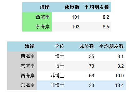

Chap 6 概率

6.2 条件概率

import random

def random_kid():
    return random.choice(['boy', 'girl'])

both_girls = 0
older_girl = 0
either_girl = 0

random.seed(100)
for _ in range(1000):
    younger = random_kid()
    older = random_kid()
    if older == 'girl':
        older_girl += 1
    if older ==  younger == 'girl':
        both_girls += 1
    if older == 'girl' or younger == 'girl':
        either_girl += 1
        
print('P(both | older) = ', both_girls / older_girl)    # 实际值1/2
print('P(both | either) = ', both_girls / either_girl)  # 实际值1/3

# P(both | older) =  0.5078740157480315
# P(both | either) =  0.35294117647058826

6.6 正态分布

import numpy as np
def normal_pdf(x, mu=0, sigma=1):
    return (np.exp(-((x - mu) / sigma) ** 2 / 2)/(np.sqrt(2 * np.pi * sigma)))

import matplotlib.pyplot as plt
from pylab import *

xs = [x / 10 for x in range(-50, 50)]
plt.plot(xs, [normal_pdf(x) for x in xs], 'c-', label='mu=0, sigma=1');
plt.plot(xs, [normal_pdf(x, sigma=2) for x in xs], 'm--', label='mu=0, sigma=2');
plt.plot(xs, [normal_pdf(x, sigma=0.5) for x in xs], 'y-.', label='mu=0, sigma=0.5');
plt.plot(xs, [normal_pdf(x, mu=-1) for x in xs], 'k:', label='mu=-1, sigma=1');
mpl.rcParams['font.sans-serif'] = ['SimHei']      # 让汉字正常显示
matplotlib.rcParams['axes.unicode_minus']=False  # 让负号正常显示
plt.title('多个正态分布概率密度函数')
plt.legend()
plt.show()

"""标准正态分布的累积分布函数无法用‘基本’的解析形式表示，但是在python中可以用函数math.erf描述"""

import math
def normal_cdf(x, mu=0, sigma=1):
    return (1 + math.erf((x - mu) / math.sqrt(2) / sigma)) / 2

xs = [x / 10 for x in range(-50, 50)]
plt.plot(xs, [normal_cdf(x) for x in xs], 'c-', label='mu=0, sigma=1');
plt.plot(xs, [normal_cdf(x, sigma=2) for x in xs], 'm--', label='mu=0, sigma=2');
plt.plot(xs, [normal_cdf(x, sigma=0.5) for x in xs], 'y-.', label='mu=0, sigma=0.5');
plt.plot(xs, [normal_cdf(x, mu=-1) for x in xs], 'k:', label='mu=-1, sigma=1');
plt.title('多个正态分布累积分布函数')
plt.legend(loc=4) # 底部右侧
plt.show()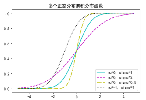

$$ erf 是误差函数， erfc是误差互补函数，erf + erfc = 1 $$

$$ erf(x) = \frac{2}{\sqrt{\pi}} \int_{0}^{x} e^{-u^2}du = \frac{2}{\sqrt{2\pi}} \int_{0}^{x} e^{-\frac{u^2}{2}}du 
          = \frac{2}{\sqrt{2\pi}} (\phi(x) - 0.5) $$
$$ erfc(x) = 1 - erf(x) = \frac{2}{\sqrt{\pi}} \int_{x}^{\infty} e^{-u^2}du $$
$$ 2 \sqrt{\pi} = \int_{-\infty}^{\infty} e^{-\frac{u^2}{2}}du $$
$$ \sqrt{\pi} = \int_{-\infty}^{\infty} e^{-u^2}du $$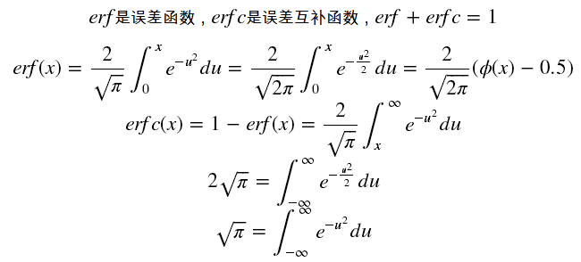

# 有时候需要对normal_cdf求逆，使用二分法查找

def inverse_normal_cdf(p, mu=0, sigma=1, tolerance=0.00001):
    # 如果非标准型，先调整单位使之服从标准型
    if mu != 0 or sigma != 1:
        return mu + sigma * inverse_normal_cdf(p, tolerance=tolerance)
    
    low_z, low_p = -10, 0   # normal_cdf(-10) -> 0
    hi_z, hi_p   = 10, 1    # normal_cdf(10) -> 1
    while hi_z - low_z > tolerance:
        mid_z = (low_z + hi_z) / 2   # midpoint
        mid_p = normal_cdf(mid_z)    # 考虑cdf在那里的值
        if mid_p < p:
            # midpoint仍然太低，搜索比他大的值
            low_z, low_p = mid_z, mid_p
        elif mid_p > p:
            # midpoint仍然太高，搜索比他小的值
            hi_z, hi_p = mid_z, mid_p
        else:
            break
            
    return mid_z

inverse_normal_cdf(0.95, mu=0, sigma=1, tolerance=0.00001)   # 1.6448

6.7 中心极限定理

# 等于1的概率是p， 等于零的概率是1-p
import random
def bernouli_trial(p):
    return 1 if random.random() < p else 0

def binomial(n, p):
    return sum(bernouli_trial(p) for _ in range(n))

# 二项分布的极限是正态，可由图像表示

import matplotlib.pyplot as  plt
from collections import Counter

def make_hist(p, n, num_points):
    
    data = [binomial(n, p) for _ in range(num_points)]
    
    # 用条形图绘出实际的二项式样本
    histogram = Counter(data)
    plt.bar([x - 0.4 for x in histogram.keys()],
            [v / num_points for v in histogram.values()],
            0.8, color='0.75')    
    mu = p * n
    sigma = math.sqrt(n * p *(1 - p))
    
    # 用线形图绘出正态近似
    xs = range(min(data), max(data) + 1)
    ys = [normal_cdf(i + 0.5, mu, sigma) - normal_cdf(i - 0.5, mu, sigma) for i in xs]
    plt.plot(xs, ys)
    
    plt.title('二项分布与正态近似')
    plt.show()

make_hist(0.75, 100, 10000)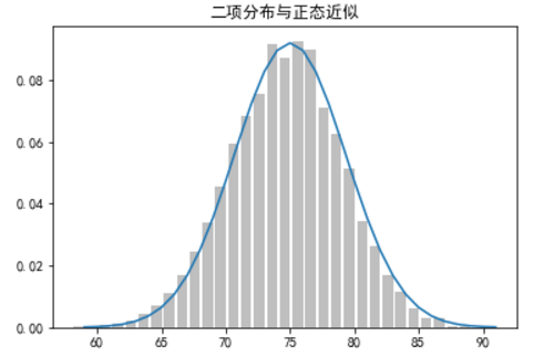

Chap 7 假设与推断

7.2 案例 ：掷硬币

def normal_approximation_to_binomial(n, p):
    mu = n * p
    sigma = np.sqrt(n * p * (1 - p))
    return mu, sigma

# 求某个区间的概率
normal_probability_below = normal_cdf
def normal_probability_above(lo, mu=0, sigma=0):
    return 1 - normal_cdf(lo, mu, sigma)

def normal_probability_between(lo, hi, mu=0, sigma=1):
    return normal_cdf(hi, mu, sigma) - normal_cdf(lo, mu, sigma)

def normal_probability_outside(lo, hi, mu=0, sigma=1):
#     return normal_cdf(lo, mu, sigma) + 1 - normal_cdf(hi, mu, sigma)
    return 1 - normal_probability_between(lo, hi, mu, sigma)

def normal_upper_bound(probability, mu=0, sigma=1):
    """return the z for which P(Z <= z) = probability"""
    return inverse_normal_cdf(probability, mu, sigma)

def normal_lower_bound(probability, mu=0, sigma=1):
    """return the z for which P(Z >= z) = probability"""
    return inverse_normal_cdf(1 - probability, mu, sigma)

# 以均值为中心两端覆盖相同的概率
def normal_two_sided_bounds(probability, mu=0, sigma=1):
    """return the symmetric (about the mean) bounds that contain the specified probability"""
    tail_probability = (1 - probability) / 2
    
    # 上界应有在它之上的tail_probability
    upper_bound = normal_lower_bound(tail_probability, mu, sigma)
    # 下界应有在它之下的tail_probability
    lower_bound = normal_upper_bound(tail_probability, mu, sigma)    
    return lower_bound, upper_bound

mu_0, sigma_0 = normal_approximation_to_binomial(1000, 0.5)
normal_two_sided_bounds(0.95, mu_0, sigma_0)
# (469.01026640487555, 530.9897335951244)

"""势（power）指的是不犯第二类错误的概率"""
lo, hi = normal_two_sided_bounds(0.95, mu_0, sigma_0)
mu_1, sigma_1 = normal_approximation_to_binomial(1000, 0.55)
type_2_probability = normal_probability_between(lo, hi, mu_1, sigma_1)
power = 1- type_2_probability
power   # 0.8865

# 左边检验
hi = normal_upper_bound(0.95, mu_0, sigma_0)
type_2_probability = normal_probability_below(hi, mu_1, sigma_1)
power = 1- type_2_probability
print('hi =',hi, 'power =',power)
# hi = 526.0073585242053 power = 0.9363794803307173

def two_sided_p_value(x, mu=0, sigma=1):
    if x >= mu:
        return 2 * normal_probability_above(x, mu, sigma)
    else:
        return 2 * normal_probability_below(x, mu, sigma)
    

# 希望看到的结果有530次正面朝上，用529.5是连续性修正    
two_sided_p_value(529.5, mu_0, sigma_0)   # 0.0062

extreme_value_count = 0
for _ in range(100000):
    num_heads = sum(1 if random.random() > 0.5 else 0 for _ in range(1000))
    if num_heads >= 530 or num_heads <= 470:
        extreme_value_count += 1
        
print(extreme_value_count / 100000)   # 0.0612

# 单边检验
upper_p_value = normal_probability_above
lower_p_value = normal_probability_below

# 525正面
print(upper_p_value(524.5, mu_0, sigma_0))   # 0.0606
 
# 527正面
print(upper_p_value(526.5, mu_0, sigma_0))   # 0.0468

7.3 置信区间

p_hat = 525 / 1000
mu = p_hatsigma = np.sqrt(p_hat * (1 - p_hat) / 1000)
normal_two_sided_bounds(0.95, mu, sigma)
# 因为0.5在区间内，我们无法得到硬币不均匀的结论
# (0.4940490278129096, 0.5559509721870904)

"""1000次抛硬币，540次正面，求估计值0.40的精度，95%置信区间"""
p_hat = 540 / 1000
mu = p_hatsigma = np.sqrt(p_hat * (1 - p_hat) / 1000)
normal_two_sided_bounds(0.95, mu, sigma)
# 因为0.5不在区间内，所以可以得到硬币不均匀的结论
# (0.5091095927295919, 0.5708904072704082)

7.5 案例：运行A/B测试

def estimated_parmeters(N, n):
    p = n / N
    sigma = np.sqrt(p * (1 - p) / N)
    return p, sigma

def a_b_test_statistic(N_A, n_A, N_B, n_B):
    p_A, sigma_A = estimated_parmeters(N_A, n_A)
    p_B, sigma_B = estimated_parmeters(N_B, n_B)
    return (p_B - p_A) / np.sqrt(sigma_A ** 2 + sigma_B ** 2)   # -1.14034

"""比较两个广告,‘口味好’点击200/1000， ‘营养均衡’点击180/1000"""
z = a_b_test_statistic(1000, 200, 1000, 180)
two_sided_p_value(z)   # 0.25414

"""比较两个广告,‘口味好’点击200/1000， ‘营养均衡’点击180/1000"""
z = a_b_test_statistic(1000, 200, 1000, 150)
two_sided_p_value(z)   # 0.0031

以上是Ch4-Ch7的相关内容

2018.03.5   YR