多目标进化算法(MOEA)概述

多目标进化算法系列
1. 多目标进化算法(MOEA)概述
2. 多目标优化-测试问题及其Pareto前沿
3. 多目标进化算法详述-MOEA/D与NSGA2优劣比较
4. 多目标进化算法-约束问题的处理方法

---

对于大多数多目标优化问题，其各个目标往往是相互冲突的，因此不可能使得所有的目标同时达到最优，而是一组各个目标值所折衷的解集，称之为Pareto最优集。以下为一些基本定义(以最小化优化问题为例)：

Definition 1: 多目标优化问题(multi-objective optimization problem(MOP))
$F(x)=(f_1(x),…,f_m(x))\\ s.t. \; x\in \Omega$

Definition 2: Pareto支配(Pareto Dominance)
x支配y,记为 x $\prec$ y ，当且仅当$\forall {i} \in \{1,2,...,m\}$,$f_i(x) \leq f_i$(y), 且$\exists {j} \in \{1,2,...,m\}$, s.t. $\; f_j(x)<f_j(y)$ 。

Definition 3: Pareto最优解(Pareto Optimal Solution)
如果一个解$x^*$ 被称之为Pareto optimal solution， 当且仅当 $x^*$ 不被其他的解支配。

Definition 4: Pareto 集(Pareto Set)
一个MOP，对于一组给定的最优解集，如果这个集合中的解是相互非支配的，也即两两不是支配关系，那么则称这个解集为Pareto Set 。

Definition 5: Pareto 前沿(Pareto Front)
Pareto Set 中每个解对应的目标值向量组成的集合称之为Pareto Front, 简称为PF

Definition 6：近似集(Approximation Set)
一般来说，准确的Pareto Set是很难得到的，其近似集相比来说容易得到，因此一般我们只需用一定数量的Approximation Set 来表示PS 。

Definition 7： 近似前沿(Approximation Front)
Approximation Set 中每个解对应的目标值向量组成的集合称之为Approximation Front 。

目前来说，由于多目标问题的复杂性，传统的数学方法不能取得较为理想的结果，而进化算法在多目标优化问题上得到了很广泛的应用，通过种群的不断进化迭代，进化算法能得到一个Approximation Set，那么我们如何来评价得到的Approximation Set的优劣呢，以下为两方面的评价标准。
Definition 7：收敛性(Convergence)
Approximation Front 与 PF 的贴近程度。

Definition 8: 分布性(Distribution)
描述Approximation Front 在PF 的分布情况，包括多样性(Diversity)和均匀性(Uniformity)。

扫描二维码关注公众号，回复： 2832764 查看本文章

具体来说，常用的两个指标分别是IGD(Inverted Generational Distance) 和 HV(Hypervolume)。其中，IGD需要知道PF数据，且其具体计算为每个PF中的点到其最近的Approximation Front中的点的距离之和的均值。同时，需注意，这两种方法都能同时度量解的分布性和收敛性。

现在来讲讲主流的多目标进化算法。
从进化算法的角度来讲，目前已有遗传算法(GA)，粒子群算法(PSO)，蚁群算法(ACO)等一系列算法用来解决多目标优化问题，但用的比较多的还是遗传算法，粒子群算法也有。
从多目标问题本身来说，主要分类如下：
- 基于Pareto支配关系
- 基于分解的方法
- 基于Indicator方法

先来介绍下基于遗传算法的多目标优化算法的一些基本参数：
种群大小：每次迭代都需保证种群大小是一致的，且其大小应由初始化设定。
交叉概率：用于衡量两个个体交叉的概率。
突变率：交叉产生的解发生突变的概率。
标准的遗传算法每次迭代都会将上一代的个体丢弃，虽然这符合自然规律，但对于遗传算法来说，这样效果不是特别好，因此，精英保留策略将上一代个体和当前个体混合竞争产生下一代，这种机制能较好的保留精英个体。
基于Pareto支配关系
最经典的方法是NSGA-II，该方法由Kalyanmoy Deb等人于2002年提出(A Fast and Elitist Multiobjective Genetic Algorithm:
NSGA-II)，该方法主要包括快速非支配排序，将每次交叉突变产生的解和前一代的解合并，然后利用非支配排序分层，其伪代码如下：

---

快速非支配排序算法流程
输入：父代子代个体构成的种群$P$
FOR each $p\in P$
$\quad$ $S_p=\varnothing$
$\quad$ $n_p=0$
$\quad$ FOR each $q\in P$
$\qquad$ IF $p\prec q$
$\quad$$\qquad$ $S_p=S_p\bigcup \{q\}$
$\qquad$ ELSEIF $q\prec p$
$\quad$ $\qquad$ $n_p=n_p+1$
$\qquad$ ENDIF
$\quad$ ENDFOR
$\quad$ IF $n_p==0$
$\qquad$ $p_{rank}=1$
$\qquad$ $F_1=F_1\bigcup \{p\}$
$\quad$ ENDIF
ENDFOR
$i=1$
WHILE $F_i\neq \varnothing$
$\quad$ $Q=\varnothing$
$\quad$ FOR each $p\in F_i$
$\qquad$ FOR each $q\in S_p$
$\quad$ $\qquad$ $n_q=n_q-1$
$\quad$ $\qquad$ IF $nq==0$
$\qquad$ $\qquad$ $q_{rank}=i+1$
$\qquad$ $\qquad$ $Q=Q\bigcup \{q\}$
$\quad$ $\qquad$ ENDIF
$\qquad$ ENDFOR
$\quad$ ENDFOR
$\quad$ $i=i+1$
$\quad$ $F_i=Q$
ENDWHILE
输出：$F_1,F_2,...,F_i$

---

再就是把每层相加直到超过种群个体，也即满足$l=argmin_l{\sum_{i=1}^{l}}>N$ 并且有 $\sum_{i=1}^{l-1}<N$， 再在第$l$层基于拥挤距离来选择解，拥挤距离伪代码如下：

---

拥挤距离计算方法
输入：第$i$层的解$Rt=F_l$
$r=|Rt|$
for each $j$,set $Rt[j]_{distance}=0$
FOR each objective $m$
$\quad$ $Rt=sort(Rt,m)$
$\quad$ $Rt[1]_{distance}=Rt[r]_{distance}=\infty$
$\quad$ FOR $j=2:(r-1)$
$\qquad$ $Rt[j]_{distance}=Rt[j]_{distance}+(Rt[j+1].m-Rt[j-1].m)/(f_m^{max}-f_m^{min})$
$\quad$ ENDFOR
ENDFOR

---

具体来说，NSGA-II使用快速非支配排序来保证收敛性，并且利用拥挤距离来保证分布性。特别说下，在迭代后期，大多数解都是非支配的，也即大多数解都在第一层。
当然，随着NSGA-II的提出，很多基于此的算法如雨后春笋般大量涌现，特别是在处理高维多目标优化问题时这种想法得到很多的应用，如VaEA，RVEA，NSGA-III等。
同时，SPEA2也是基于Pareto支配关系的一种较为流行的算法(SPEA2: Improving the Strength Pareto Evolutionary Algorithm)，该算法使用一个外部保存集来保存较为优秀的解，同时，对每一个解，利用其支配的解的数量和基于KNN的邻近解的距离来给每一个解打分，得分越小的解更优。

基于分解的方法
该方法第一次系统地被提出是在2007年由Qingfu Zhang等人提出(MOEA/D: A Multiobjective Evolutionary Algorithm Based on Decomposition)，该方法将MOP分解为多个子问题，这样就可以优化每个子问题来求解一个MOP。一般而言，基于分解的方法首先需要得到一组均匀分布的参照向量来指导选择操作。在此，有必要说说产生参照向量的方法。目前对于低维多目标优化问题，常用方法为Das and Dennis于1998年提出的systematic approach(Normal-boundary intersection: A new method for generating the pareto surface in nonlinear multicriteria optimization problems).
对于每个参照向量，其指导选择的过程需要比较解的优劣，这就需要用到一些标量函数来定量衡量一个解对于这个参照向量的适应度值。常用的标量函数包括：
- Weighted Sum Approach
- Tchebycheff Approach
- penalty-based boundary intersection (PBI) approach

Weighted Sum Approach
$min \; g^{ws}(x|\lambda)=\sum_{i=1}^m\lambda_if_i(x)$
其中$\lambda$是参照向量，其运行机理如下图：

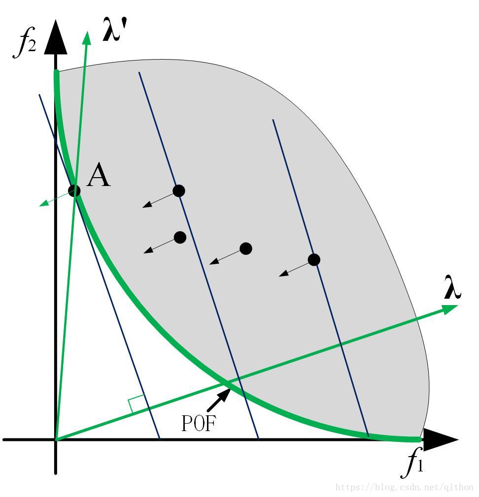
这里需要注意，标准的Weighted Sum Approach不能处理非凸问题，因为由上图可知，对于非凸问题，每个参照向量的垂线与其前沿不可能相切。对于这个问题，Rui Wang等人与2016年提出相对应的改进(Localized weighted sum method for many-objective optimization)，主要是约束替换范围。

Tchebycheff Approach
$min\; g^{te}(x|\lambda,z^*)=max\; \{\lambda_i (f_i(x) - z_i^*)\}$
其中$\lambda$是参照向量，其运行机理如下图：

标准的Tchebycheff Approach得到的解不均匀，为此Yutao Qi等人于2014年提出一种解决方法(MOEA/D with Adaptive Weight Adjustment)，$\lambda^* =(\frac{\frac{1}{\lambda_1}}{\sum_{i=1}^m\frac{1}{\lambda_i}},....,\frac{\frac{1}{\lambda_m}}{\sum_{i=1}^m\frac{1}{\lambda_i}})$,通过这个参照向量的转换即可得到分布均匀的解。

penalty-based boundary intersection (PBI) approach
$min\; g^{pbi}(x|\lambda,z^*)=d_1+\theta d_2$

其中$d_1$，$d_2$如上图所示。一般来说，$\theta = 5$是比较常用的，Yuan Yuan等人提出的$\theta -DEA$算法对$\theta$的取值有较为详细的讨论(A New Dominance Relation-Based Evolutionary Algorithm for Many-Objective Optimization)。
基于分解的进化方法框架如下：

---

MOEA/D算法流程

$N$个均匀分布的权重向量：$\lambda_1,\lambda_2,...,\lambda_N$ // $N$ 是种群大小
$P_0$：随机初始化的种群
$z^*$：初始化的理想点
$T$：每个权重向量的邻居的个数
$B(i)=(i_1,i_2,...,i_T)$是第$i$个权重向量的$T$个邻居的编号
$t = 0$
WHILE $t < MaxIteration$
$\quad$ FOR($i=1,2,...,N$)
$\qquad$构造新解：从$B(i)$中随机选择两个索引$k,l$，再基于$x^k,x^l$生成新解$y$
$\qquad$更新$z^*$：对于$j=1,2,...,m$,如果$z_j^*<f)j(y)$，则用$f_j(y)$取代$z_j^*$
$\qquad$更新近邻解：对于每一个$j\in B(i)$，如果$g(y|\lambda_j,z^*)\leq g(x^j|\lambda_j,z^*)$，那么则用解$y$取代$x^j$
$\quad$ ENDFOR
$\quad$$t = t + 1$
ENDWHILE
输出结果

---

基于Indicator方法
相比于IGD指标，Hypervolume更容易用来作为一个测度在种群进化过程中用来选择个体,如IBEA[8]以及其快速计算HV的HypE[9]，因为IGD需要知道真实的Pareto Front数据，而这对于一个未知多目标优化问题是相当困难的，但有些算法是用当前的非支配解来近似Pareto Front，如AR-MOEA[10]。

至于具体的多目标进化算法后续将会详细介绍。

QQ交流群：399652146

参考文献
[1] K. Deb, A. Pratap, S. Agarwal, and T. Meyarivan, “A fast and elitist multiobjective genetic algorithm: NSGA-II,” IEEE Trans. Evol. Comput., vol. 6, no. 2, pp. 182–197, Apr. 2002
[2] E. Zitzler, M. Laumanns, and L. Thiele, “SPEA2: Improving the strength Pareto evolutionary algorithm,” in Proc. Evol. Methods Design Optim. Control Appl. Ind. Prob., Athens, Greece, 2002, pp. 95–100.
[3] Qingfu Zhang and Hui Li. Moea/d: A multiobjective evolutionary algorithm based on decomposition. IEEE Transactions on evolutionary computation, 11(6):712–731, 2007.
[4] Yutao Qi, Xiaoliang Ma, Fang Liu, Licheng Jiao, Jianyong Sun, and Jianshe Wu. MOEA/D with adaptive weight adjustment. Evolutionary computation, 22(2):231–264, 2014.
[5] Kalyanmoy Deb and Himanshu Jain. An evolutionary many objective optimization algorithm using reference- point-based nondominated sorting approach, part i: Solving problems with box constraints. IEEE Trans. Evolutionary Computation, 18(4):577–601, 2014.
[6] Yuan Yuan, Hua Xu, Bo Wang, and Xin Yao. A new dominance relation-based evolutionary algorithm for many-objective optimization. IEEE Transactions on Evolutionary Computation, 20(1):16–37, 2016.
[7] Indraneel Das and John E Dennis. Normal-boundary intersection: A new method for generating the pareto surface in nonlinear multicriteria optimization problems. SIAM Journal on Optimization, 8(3):631–657, 1998
[8] E. Zitzler and S. Kunzli, “Indicator-based selection in multiob- jective search,”in Proceedings of the 8th International Conference on Parallel Problem Solving from Nature, 2004, pp. 832–842.
[9] J. Bader and E. Zitzler, “HypE: An algorithm for fast hypervolume-based many-objective optimization,” Evolutionary Computation, vol. 19, no. 1, pp. 45–76, 2011.
[10] Tian Y, Cheng R, Zhang X, et al. An Indicator Based Multi-Objective Evolutionary Algorithm with Reference Point Adaptation for Better Versatility[J]. IEEE Transactions on Evolutionary Computation, 2017, PP(99):1-1.
[11] 张作峰. 基于分解的多目标进化算法研究[D]. 湘潭大学, 2013.