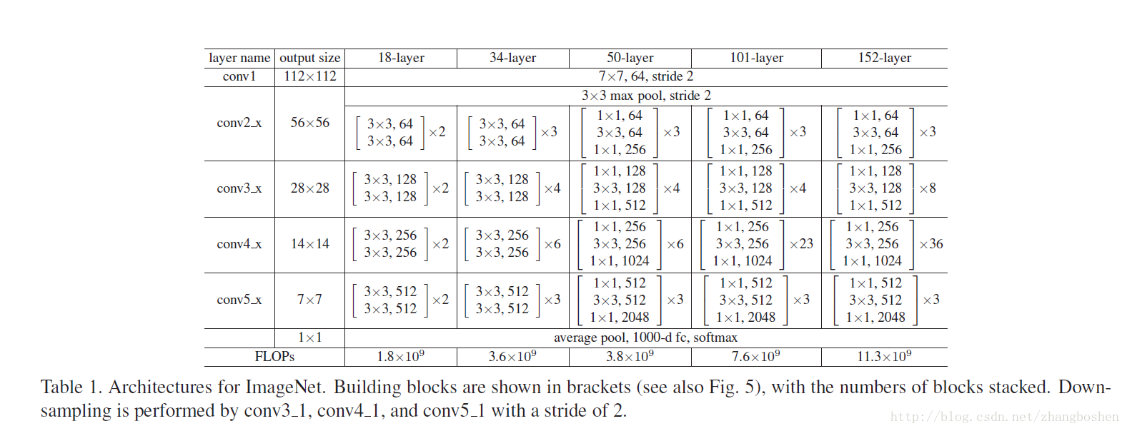
ResNet自从15年问世以来迅速影响了CNN的发展,主要得益于ResNet的shortcut结构能够避免网络的退化(即传统的CNN随着网络深度的 增加会出现训练误差和测试误差增大的情况)和梯度消失/爆炸现象,使得ResNet能够从网络层数的加深中受益,这也是为什么ResNet 能够做到34层,50层,甚至152层,甚至是1202层的缘故。原文中提供了几个通用的网络结构:
本文分析GitHub上面的TensorFlow提供的官方ResNet的TensorFlow实现程序,讲解网络在TensorFlow中的代码构成。
首先这是对ResNet在Cifar10和Cifar100数据库的一个复现,也就是说TensorFlow官方提供的这一版ResNet程序是用来进行Cifar的分类任务的。代码地址:https://github.com/tensorflow/models
cifar_input.py(https://github.com/tensorflow/models/blob/master/resnet/cifar_input.py)
用来读取Cifar数据库中的图片数据和标注信息的,这里不做过多讲解,如果想要把ResNet改为回归任务或者是训练自己的数据库,则需要对数据输入进行重写(如果是回归任务,那么网络的结构也需要修改(去掉Softmax层)
resnet_model.py(https://github.com/tensorflow/models/blob/master/resnet/resnet_model.py)
构造了ResNet这个类(Class),定义了ResNet的网络结构、loss等。
首先_build_model()函数定义了网络的核心结构,代码如下:
def _build_model(self):
    """Build the core model within the graph."""
    with tf.variable_scope('init'):    #init层将图片的3通道变为16通道feature map输出
      x = self._images
      x = self._conv('init_conv', x, 3, 3, 16, self._stride_arr(1))  #3*3的卷积层,16通道输出

    strides = [1, 2, 2]   #后面两个2的stride用来降采样
    activate_before_residual = [True, False, False]
    if self.hps.use_bottleneck:
      res_func = self._bottleneck_residual    #bottleneck结构,包含三个卷积子层
      filters = [16, 64, 128, 256]
    else:
      res_func = self._residual      #非bottleneck结构(包含两个3*3的卷积子层)
      filters = [16, 16, 32, 64]
      # Uncomment the following codes to use w28-10 wide residual network.
      # It is more memory efficient than very deep residual network and has
      # comparably good performance.
      # https://arxiv.org/pdf/1605.07146v1.pdf
      # filters = [16, 160, 320, 640]
      # Update hps.num_residual_units to 9

    with tf.variable_scope('unit_1_0'):
      x = res_func(x, filters[0], filters[1], self._stride_arr(strides[0]),
                   activate_before_residual[0])
    for i in six.moves.range(1, self.hps.num_residual_units):   #可以看到这里num_residual_units决定了一个unit下面包含几个block
      with tf.variable_scope('unit_1_%d' % i):
        x = res_func(x, filters[1], filters[1], self._stride_arr(1), False)

    with tf.variable_scope('unit_2_0'):
      x = res_func(x, filters[1], filters[2], self._stride_arr(strides[1]),
                   activate_before_residual[1])
    for i in six.moves.range(1, self.hps.num_residual_units):
      with tf.variable_scope('unit_2_%d' % i):
        x = res_func(x, filters[2], filters[2], self._stride_arr(1), False)

    with tf.variable_scope('unit_3_0'):
      x = res_func(x, filters[2], filters[3], self._stride_arr(strides[2]),
                   activate_before_residual[2])
    for i in six.moves.range(1, self.hps.num_residual_units):
      with tf.variable_scope('unit_3_%d' % i):
        x = res_func(x, filters[3], filters[3], self._stride_arr(1), False)

    with tf.variable_scope('unit_last'):      #卷积完成之后有一个全局Pooling层
      x = self._batch_norm('final_bn', x)
      x = self._relu(x, self.hps.relu_leakiness)
      x = self._global_avg_pool(x)

    with tf.variable_scope('logit'):
      logits = self._fully_connected(x, self.hps.num_classes)    #全连接层输出
      self.predictions = tf.nn.softmax(logits)           #Softmax分类输出结果

    with tf.variable_scope('costs'):
      xent = tf.nn.softmax_cross_entropy_with_logits(    #损失函数采用的Softmax交叉熵的形式
          logits=logits, labels=self.labels)
      self.cost = tf.reduce_mean(xent, name='xent')
      self.cost += self._decay()

      tf.summary.scalar('cost', self.cost)      #summary收集信息用于tensorboard的可视化显示
此外,ResNet类中还采用BN的算法一个weight decay的算法,也都在resnet_model.py中有定义。
resnet_main.py(https://github.com/tensorflow/models/blob/master/resnet/resnet_main.py) 是训练代码和测试代码。训练代码中的 _LearningRateSetterHook类定义了学习率随迭代次数的变化而变化:
 class _LearningRateSetterHook(tf.train.SessionRunHook):
    """Sets learning_rate based on global step."""

    def begin(self):
      self._lrn_rate = 0.1

    def before_run(self, run_context):
      return tf.train.SessionRunArgs(
          model.global_step,  # Asks for global step value.
          feed_dict={model.lrn_rate: self._lrn_rate})  # Sets learning rate

    def after_run(self, run_context, run_values):
      train_step = run_values.results
      if train_step < 40000:
        self._lrn_rate = 0.1
      elif train_step < 60000:
        self._lrn_rate = 0.01
      elif train_step < 80000:
        self._lrn_rate = 0.001
      else:
        self._lrn_rate = 0.0001
主函数中定义了超参数的各项设置:
def main(_):
  if FLAGS.num_gpus == 0:
    dev = '/cpu:0'
  elif FLAGS.num_gpus == 1:
    dev = '/gpu:0'
  else:
    raise ValueError('Only support 0 or 1 gpu.')

  if FLAGS.mode == 'train':
    batch_size = 128
  elif FLAGS.mode == 'eval':
    batch_size = 100

  if FLAGS.dataset == 'cifar10':
    num_classes = 10
  elif FLAGS.dataset == 'cifar100':
    num_classes = 100

  hps = resnet_model.HParams(batch_size=batch_size,
                             num_classes=num_classes,
                             min_lrn_rate=0.0001,
                             lrn_rate=0.1,
                             num_residual_units=5,
                             use_bottleneck=False,
                             weight_decay_rate=0.0002,
                             relu_leakiness=0.1,
                             optimizer='mom')

  with tf.device(dev):
    if FLAGS.mode == 'train':
      train(hps)
    elif FLAGS.mode == 'eval':
      evaluate(hps)
前面提到过,num_residual_units用来定义一个unit下面的block数量,这里设为5;use_bottleneck=False表示不使用bottleneck结构,即一个block下面只包含两个卷积子层;好了,这里规定num_residual_units和use_bottleneck之后,实际上网络结构就确定了;这个网络长什么样子呢,这里给出一个上面的超参数设置所对用的可视化的网络结构:
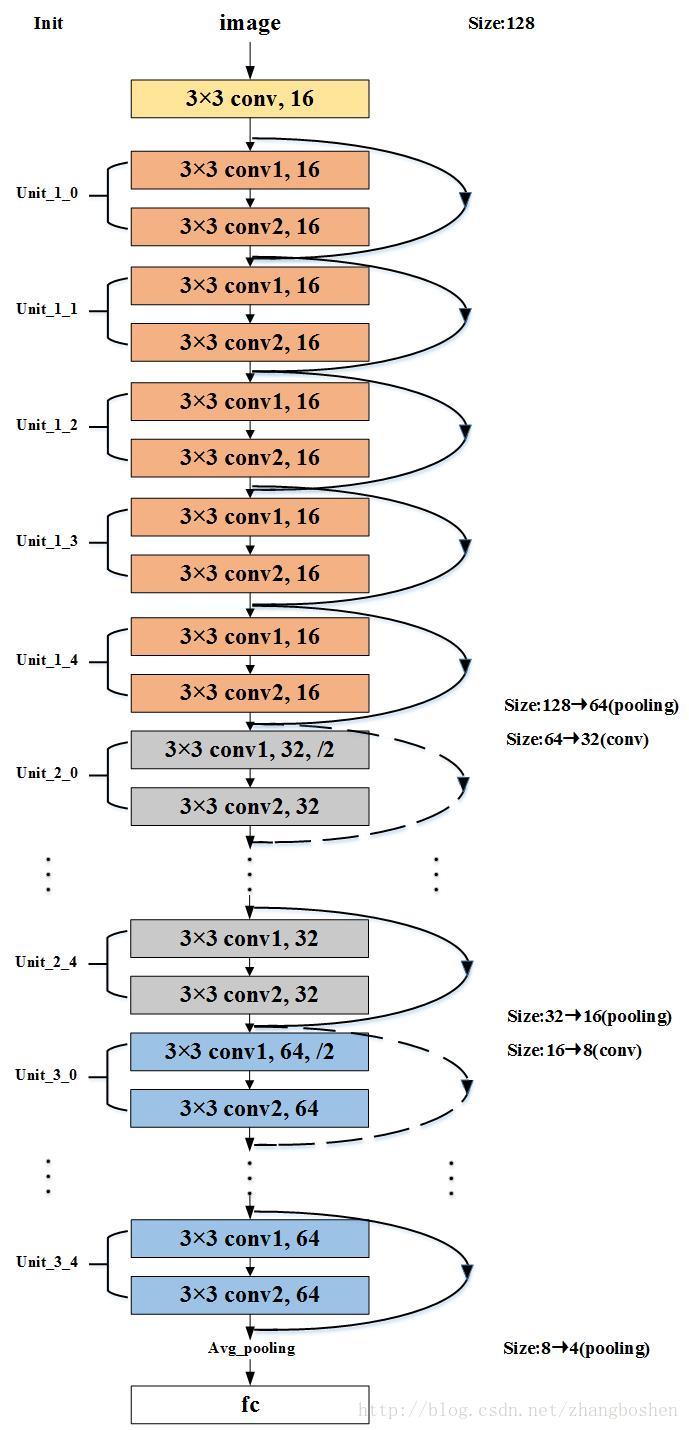
图中不同填充颜色的方框代表不同的unit,这是一个包含32个参数层(卷积层和全连接层)的网络结构,每一个Block包含conv1和con2两个子层,属于一个浅层的ResNet。
如果想要设计自己的ResNet用于不同的任务,需要修改训练数据的输入部分以及部分网路结构,最简单的,num_residual_units这个参数就可以控制网络总的深度:
网络层数 = 2*3*num_residual_units+2;(当use_bottleneck = False时)
此外,use_bottleneck = True时采用的bottleneck结构每一个block包含三个卷积子层,不同于上面的网络结构,按照原文的说法,这种bottleneck结构应该更容易优化和利于网络的加深,原文中给出的50层、101层、152层网络事实上都是采用的这种结构,非bottleneck结构一般来说只在浅层ResNet中使用。