kaggle是一个很好的数据分析挖掘项目平台。可以从中感受到数据分析挖掘的实际应用价值,锻炼技能。它还是一个社交平台。
项目介绍:
在数据分析挖掘的过程中,最重要的一步就是提出重要的问题。
这一步做不好,接下来数据再好,分析在精妙,也没有意义(这也是统计的三要素:问题、数据、方法)。
银行在现代经济生活中扮演至关重要的地位,它希望借贷出去更多款项,但同时它又必须确保借贷人有偿还能力。这就涉及到金融风险预测评估的问题。根据历史,预测未来。根据历史数据,来预测未来会不会发生信用违约的情况,这是一个很重要的数据分析挖掘应用方向。以数据为依据,辅导决策!
数据介绍:
数据来源:give me some credit-kaggle
| Variable Name | Description | Type |
| SeriousDlqin2yrs | Person experienced 90 days past due delinquency or worse 是否有超过90天或更长时间逾期未还的不良行为 | Y/N |
| RevolvingUtilizationOfUnsecuredLines不安全额度循环利用 | Total balance on credit cards and personal lines of credit except real estate and no installment debt like car loans divided by the sum of credit limits.信用卡总余额和个人信用额度(除了房地产和分期付款给债务,比如汽车贷款)除以总信用限制。 | percentage |
| age | Age of borrower in years借贷者的年龄(以年计) | integer |
| NumberOfTime30-59DaysPastDueNotWorse | Number of times borrower has been 30-59 days past due but no worse in the last 2 years. | integer |
| DebtRatio | Monthly debt payments, alimony,living costs divided by monthy gross income月债务支出、赡养费、生活费除以总收入(毛收入) | percentage |
| MonthlyIncome | Monthly income | real |
| NumberOfOpenCreditLinesAndLoans | Number of Open loans (installment like car loan or mortgage) and Lines of credit (e.g. credit cards)公开贷款(如汽车和抵押的分期)和信用上线(比如信用卡)数量 | integer |
| NumberOfTimes90DaysLate | Number of times borrower has been 90 days or more past due(应付款、应付日期).90天或以上贷款者逾期未还的次数。 | integer |
| NumberRealEstateLoansOrLines | Number of mortgage and real estate loans including home equity lines of credit抵押和房地产数量(包括房屋净值信用额度) | integer |
| NumberOfTime60-89DaysPastDueNotWorse | Number of times borrower has been 60-89 days past due but no worse in the last 2 years. | integer |
| NumberOfDependents | Number of dependents in family excluding themselves (spouse, children etc.)家庭中的依赖者(比如说配偶子女,但不包括他自己) | integer |
数据初探:
1.弄清楚数据条数(完整性)和类型
import pandas as pd


data_train = pd.read_csv('cs-training.csv')
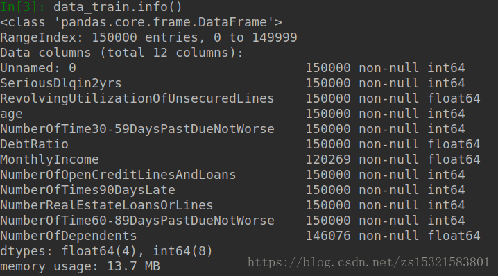
了解到月收入和亲属人数2个特征中有缺省项。
2.了解各个特征的统计信息:
如果是KAGGLE中的数据,那么它还提供各个特征数据的频数分布直方图:
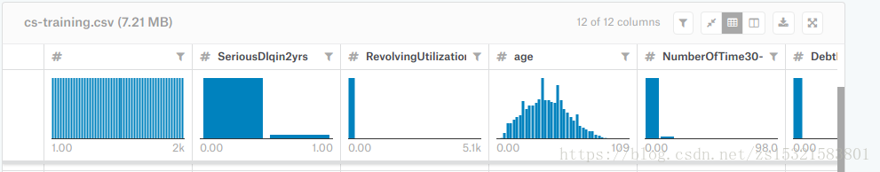
(以上截图出自pycharm,但是它的显示效果没有jupyter notebook好,后者会将结果以表格的形式显示出来!)
| Unnamed: 0 | SeriousDlqin2yrs | RevolvingUtilizationOfUnsecuredLines | age | NumberOfTime30-59DaysPastDueNotWorse | DebtRatio | MonthlyIncome | NumberOfOpenCreditLinesAndLoans | NumberOfTimes90DaysLate | NumberRealEstateLoansOrLines | NumberOfTime60-89DaysPastDueNotWorse | NumberOfDependents | |
|---|---|---|---|---|---|---|---|---|---|---|---|---|
| count | 150000.000000 | 150000.000000 | 150000.000000 | 150000.000000 | 150000.000000 | 150000.000000 | 1.202690e+05 | 150000.000000 | 150000.000000 | 150000.000000 | 150000.000000 | 146076.000000 |
| mean | 75000.500000 | 0.066840 | 6.048438 | 52.295207 | 0.421033 | 353.005076 | 6.670221e+03 | 8.452760 | 0.265973 | 1.018240 | 0.240387 | 0.757222 |
| std | 43301.414527 | 0.249746 | 249.755371 | 14.771866 | 4.192781 | 2037.818523 | 1.438467e+04 | 5.145951 | 4.169304 | 1.129771 | 4.155179 | 1.115086 |
| min | 1.000000 | 0.000000 | 0.000000 | 0.000000 | 0.000000 | 0.000000 | 0.000000e+00 | 0.000000 | 0.000000 | 0.000000 | 0.000000 | 0.000000 |
| 25% | 37500.750000 | 0.000000 | 0.029867 | 41.000000 | 0.000000 | 0.175074 | 3.400000e+03 | 5.000000 | 0.000000 | 0.000000 | 0.000000 | 0.000000 |
| 50% | 75000.500000 | 0.000000 | 0.154181 | 52.000000 | 0.000000 | 0.366508 | 5.400000e+03 | 8.000000 | 0.000000 | 1.000000 | 0.000000 | 0.000000 |
| 75% | 112500.250000 | 0.000000 | 0.559046 | 63.000000 | 0.000000 | 0.868254 | 8.249000e+03 | 11.000000 | 0.000000 | 2.000000 | 0.000000 | 1.000000 |
| max | 150000.000000 | 1.000000 | 50708.000000 | 109.000000 | 98.000000 | 329664.000000 | 3.008750e+06 | 58.000000 | 98.000000 | 54.000000 | 98.000000 | 20.000000 |
从SeriousDlqin2yrs特征的统计信息中可以看出,这个数据集是一个极度不平衡的数据。
3.各项特征与结果的关联统计
探究连续型变量对某个分类结果的影响,方法之一是先将连续型变量用cut()离散成分段变量,然后统计各分段内的某一事件发声概率。
# 数据清洗
# 删除第一列,将.csv文件导入DataFrame中后会有自动索引
df = df.drop(df.columns[0], axis=1)
# 联系实际和统计信息,发现异常数据age<18的一项
# 查看age<18的项
# df[df.age < 18]
# 去掉age<18的项
df = df[df.age > 18]

# 通过了解数据背景,知道特征为连续型变量
# 特征若是分类变量,可以将每个特征不良和正常的数据分别做成频率分布表,
# 显示在一张图表中进行对比,可以对每个特征对结果的影响进行一个直观的了解。


# 使用cut函数,将连续变量转换成分类变量
def binning(col, cut_points, labels=None, isright=True):
    val_min = col.min()
    val_max = col.max()
    break_points = [val_min] + cut_points + [val_max]
    if not labels:
        labels = range(len(cut_points) + 1)
    else:
        labels = [str(i + 1) + ':' + labels[i] for i in range(len(cut_points) + 1)]
    colbin = pd.cut(col, bins=break_points, labels=labels, include_lowest=True, right=isright)
    return colbin


# 将RevolvingUtilizationOfUnsecuredLines离散化
# 尽量不要在原始数据集中更改数据
df_tmp = df[['SeriousDlqin2yrs', 'RevolvingUtilizationOfUnsecuredLines']]

cut_points = [0.25, 0.5, 0.75, 1, 2]
labels = ['below0.25', '0.25-0.5', '0.5-0.75', '0.75-1.0', '1.0-2.0', 'above2']
df_tmp['Utilization_Bin'] = binning(df_tmp['RevolvingUtilizationOfUnsecuredLines'], cut_points, labels)

# 制作频率分布透视表
# 总人数
# total_size = df_tmp.shape[0]
# pd.pivot_table()是制作透视表工具。可以有多级索引,也可以有多级列标(如果默认column=None,那就是所有除了
# 索引外的列都是列标和计算值,列的聚合函数可以有多个。
# per_table = pd.pivot_table(df_tmp, index='Utilization_Bin', aggfunc = {'RevolvingUtilizationOfUnsecuredLines': [len, \
# lambda x:len(x)/total_size*100], 'SeriousDlqin2yrs': np.sum}, values=['RevolvingUtilizationOfUnsecuredLines','Serious\
# Dlqin2yrs'])
# per_table = pd.pivot_table(df_tmp, index=['Utilization_Bin'], aggfunc={"RevolvingUtilizationOfUnsecuredLines":[len, \
# lambda x:len(x)/total_size*100],"SeriousDlqin2yrs":[np.sum] },values=['RevolvingUtilizationOfUnsecuredLines','Seriou\
# sDlqin2yrs'])
# 给透视表增加违约率列
# 多级索引数据框的索引格式pd[a_level,b_level,..]
# per_table['SeriousDlqin2yrs', 'percent'] = per_table['SeriousDlqin2yrs', 'sum'] / per_table['RevolvingUtilizationO\
# fUnsecuredLines', 'len']*100
# 给透视表重命名
# per_table = per_table.rename(columns={'<lambda>': 'percent', 'len': 'number', 'sum': 'number'})
# 把number 放在前面,percent放在后面更合理,用reindex调整顺序
# per_table = per_table.reindex((per_table.columns[1], per_table.columns[0], per_table.columns[2], per_table.col\
# umns[3]), axis=1)
# 将上述生成频率分布表的过程写成函数,以便对每个变量进行类似处理
def get_frequency(df, col_x, col_y, cut_points, labels, isright=True):
    df_tmp = df[[col_x, col_y]]
    df_tmp['columns_Bin'] = binning(df_tmp[col_x], cut_points, labels, isright=isright)
    total_size = df_tmp.shape[0]
    per_table = pd.pivot_table(df_tmp, index='columns_Bin', aggfunc={col_x:[len, lambda x:len(x)/total_size], col_y:
        np.sum}, values=[col_x, col_y])
    if per_table.columns[0][0] != col_x:
        # 假如col_x不在第一列,说明是在第2/3列,就把他们往前挪
        per_table = per_table.reindex((per_table.columns[1], per_table.columns[2], per_table.columns[0]), axis=1)
    per_table[col_y, 'percent'] = per_table[col_y, 'sum'] / per_table[col_x, 'len']*100
    per_table = per_table.rename(columns={'<lambda>': 'percent', 'len': 'number', 'sum': 'number'})
    per_table = per_table.reindex((per_table.columns[1], per_table.columns[0], per_table.columns[2], per_table.
                                       columns[3]), axis=1)
    return per_table
上图中的行索引是将RevolvingUtilizationOfUnsecuredLines列的连续百分比值变成分段的离散变量;第一个number是分段人数统计,第一个percent是分段人数占总人数的比例;第二个number是分段内的违约人数,第二个percent是分段违约人数占总人数的比例。
从上表中可以看出变量RevolvingUtilizationOfUnsecuredLines对违约率的影响,呈不对称的钟形分布。
对其他各个特征变量与违约率的关系:
# age
cut_points = [25, 35, 45, 55, 65]
labels = ['below25', '26-35', '36-45', '46-55', '56-65', 'above65']
freq_age = get_frequency(df, 'age', 'SeriousDlqin2yrs', cut_points, labels)
# print(freq_age)

#DeptRatio
cut_points = [0.25,0.5,0.75,1,2]
labels = ["below0.25","0.25-0.5","0.5-0.75","0.75-1.0","1.0-2.0","above2"]
feq_ratio=get_frequency(df,'DebtRatio','SeriousDlqin2yrs', cut_points, labels)
#print(feq_ratio)
#NumberOfOpenCreditLinesAndLoans
cut_points=[5,10,15,20,25,30]
labels=['below 5', '6-10', '11-15','16-20','21-25','26-30','above 30']
feq_OpenCredit=get_frequency(df,'NumberOfOpenCreditLinesAndLoans','SeriousDlqin2yrs', cut_points, labels)
#print(feq_OpenCredit)
#NumberRealEstateLoansOrLines
cut_points=[5,10,15,20]
labels=['below 5', '6-10', '11-15','16-20','above 20']
feq_RealEstate=get_frequency(df,'NumberRealEstateLoansOrLines','SeriousDlqin2yrs', cut_points, labels)
#print(feq_RealEstate)
#NumberOfTime30-59DaysPastDueNotWorse
cut_points=[1,2,3,4,5,6,7]
labels=['0','1','2','3','4','5','6','7 and above',]
feq_30days=get_frequency(df,'NumberOfTime30-59DaysPastDueNotWorse','SeriousDlqin2yrs', cut_points, labels,isright=False)
#print(feq_30days)
#MonthlyIncome
cut_points=[5000,10000,15000]
labels=['below 5000', '5000-10000','1000-15000','above 15000']
feq_Income=get_frequency(df,'MonthlyIncome','SeriousDlqin2yrs', cut_points, labels)
#print(feq_Income)
#NumberOfDependents
cut_points = [1,2,3,4,5]
labels = ["0","1","2","3","4","5 and more"]
feq_dependent=get_frequency(df,'NumberOfDependents','SeriousDlqin2yrs', cut_points, labels,isright=False)
print(feq_dependent)
                age           SeriousDlqin2yrs
              number   percent           number    percent
columns_Bin
1:below25     3027.0  0.020180              338  11.166171
2:26-35      18458.0  0.123054             2053  11.122548
3:36-45      29819.0  0.198795             2628   8.813173
4:46-55      36690.0  0.244602             2786   7.593350
5:56-65      33406.0  0.222708             1531   4.583009
6:above65    28599.0  0.190661              690   2.412672
------------------------------
            DebtRatio           SeriousDlqin2yrs
               number   percent           number    percent
columns_Bin
1:below0.25   52361.0  0.349076             3126   5.970092
2:0.25-0.5    41346.0  0.275642             2529   6.116674
3:0.5-0.75    15728.0  0.104854             1484   9.435402
4:0.75-1.0     5427.0  0.036180              596  10.982126
5:1.0-2.0      4092.0  0.027280              539  13.172043
6:above2      31045.0  0.206968             1752   5.643421
------------------------------
            NumberOfOpenCreditLinesAndLoans           SeriousDlqin2yrs  \
                                     number   percent           number
columns_Bin
1:below 5                           46590.0  0.310602             3922
2:6-10                              60399.0  0.402663             3345
3:11-15                             29184.0  0.194561             1804
4:16-20                              9846.0  0.065640              676
5:21-25                              2841.0  0.018940              191
6:26-30                               785.0  0.005233               62
7:above 30                            354.0  0.002360               26


              percent
columns_Bin
1:below 5    8.418115
2:6-10       5.538171
3:11-15      6.181469
4:16-20      6.865732
5:21-25      6.722985
6:26-30      7.898089
7:above 30   7.344633
------------------------------
            NumberRealEstateLoansOrLines           SeriousDlqin2yrs
                                  number   percent           number    percent
columns_Bin
1:below 5                       149206.0  0.994713             9884   6.624398
2:6-10                             699.0  0.004660              121  17.310443
3:11-15                             70.0  0.000467               16  22.857143
4:16-20                             14.0  0.000093                3  21.428571
5:above 20                          10.0  0.000067                2  20.000000
------------------------------
              NumberOfTime30-59DaysPastDueNotWorse           SeriousDlqin2yrs  \
                                            number   percent           number
columns_Bin
1:0                                       126018.0  0.840126             5041
2:1                                        16032.0  0.106881             2409
3:2                                         4598.0  0.030654             1219
4:3                                         1754.0  0.011693              618
5:4                                          747.0  0.004980              318
6:5                                          342.0  0.002280              154
7:6                                          140.0  0.000933               74
8:7 and above                                104.0  0.000693               50


                 percent
columns_Bin
1:0             4.000222
2:1            15.026198
3:2            26.511527
4:3            35.233751
5:4            42.570281
6:5            45.029240
7:6            52.857143
8:7 and above  48.076923
------------------------------
              MonthlyIncome           SeriousDlqin2yrs
                     number   percent           number   percent
columns_Bin
1:below 5000        55859.0  0.372396             4813  8.616338
2:5000-10000        46090.0  0.307269             2752  5.970926
3:1000-15000        13035.0  0.086901              547  4.196394
4:above 15000        5284.0  0.035227              245  4.636639
------------------------------
             NumberOfDependents           SeriousDlqin2yrs
                         number   percent           number    percent
columns_Bin
1:0                     86902.0  0.579351             5095   5.862926
2:1                     26316.0  0.175441             1935   7.352941
3:2                     19521.0  0.130141             1584   8.114338
4:3                      9483.0  0.063220              837   8.826321
5:4                      2862.0  0.019080              297  10.377358
6:5 and more              990.0  0.006600               99  10.000000
将上列表格变成更直观的图形:
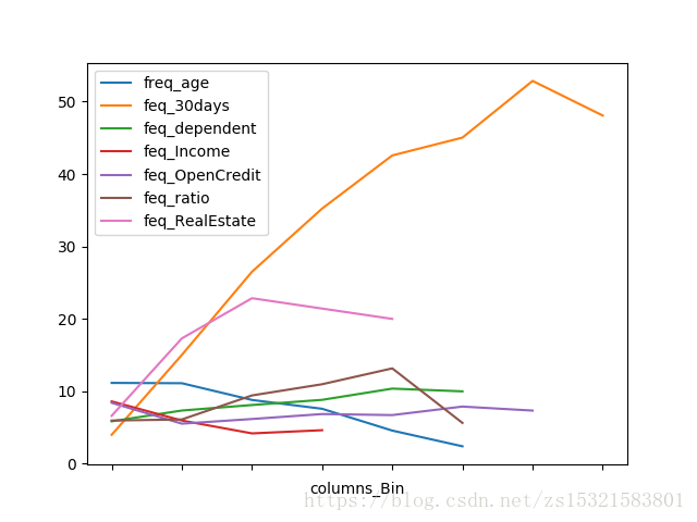
由上表统计信息可知:
1.随着年龄增加,贷款违约率降低
2.随着借贷率的升高,违约率先升后降。
3.随着30天违约次数的升高,违约率先先急剧升高后降。
4.随着亲人数的增加,违约率缓慢增加。
5.随着收入增加,违约率先缓慢降低然后基本不变。
。。。
模型构建:
比较逻辑回归模型、决策树模型和随机森林模型的AUC值,择优选用。
# coding = utf-8
import pandas as pd
import numpy as np
from sklearn.ensemble import RandomForestClassifier
from sklearn.metrics import roc_auc_score
from sklearn.model_selection import GridSearchCV
from sklearn.model_selection import StratifiedShuffleSplit
from sklearn.preprocessing import Imputer

from sklearn.linear_model.logistic import LogisticRegression
from sklearn import tree

# 忽略警告错误的输出
import warnings
warnings.filterwarnings('ignore')


# 用数据集构造随机森林分类器模型
# 加载数据(训练和测试)
# preprocessing
# split training_data into training_new&test_new to verify model
# use mean_value to replace default_value with the method Imputer
# build a RandomForestModel with training_new
# deal with the unbalanced data problem
# perform parameters'ajustment with GridSearchCV in CrossValidation
# export best model and test it with data_test

# 创建字典函数
# input: keys = [] and values = []
# output: dict{}


def create_dict(keys, vals):
    lookup = {}
    if len(keys) == len(vals):
        for i in range(len(keys)):
            key = keys[i]
            val = vals[i]
            lookup[key] = val
    return lookup


# 计算AUC函数
# input: y_true = [] and y_score = []
# output: auc


def compute_auc(y_true, y_score):
    auc = roc_auc_score(y_true, y_score)
    print('auc', auc)
    return auc

def main():
    # 1,加载数据(训练和测试)和预处理数据
    colnames = ['ID', 'label', 'RUUnsecuredL', 'age', 'NOTime30-59',
                'DebtRatio', 'Income', 'NOCredit', 'NOTimes90',
                'NORealEstate', 'NOTime60-89', 'NODependents']
    # 将数据集中没有意义的数值全部指定为‘NA',比如年龄小于18,
    col_nas = ['', 'NA', 'NA', 0, [98, 96], 'NA', 'NA', 'NA', [98, 96], 'NA', [98, 96], 'NA']    col_na_values = create_dict(colnames, col_nas)
    dftrain = pd.read_csv('cs-training.csv', names=colnames,
                          na_values=col_na_values, skiprows=[0])
    # print(dftrain)
    # pop()返回删除的列,并默认本地删除
    train_id = [int(x) for x in dftrain.pop('ID')]
    y_train = np.asarray([int(x) for x in dftrain.pop('label')])
    x_train = dftrain.values

    dftest = pd.read_csv('cs-test.csv', names=colnames,
                         na_values=col_na_values, skiprows=[0])
    test_id = [int(x) for x in dftest.pop('ID')]
    y_test = np.asarray(dftest.pop('label'))
    x_test = dftest.values

    # 2,使用StratifiedShuffleSplit将训练数据分解为trainning_new和test_new(用于验证模型)
    sss = StratifiedShuffleSplit(n_splits=1, test_size=0.33333, random_state=0)
    for train_index, test_index in sss.split(x_train, y_train):
        # print("TRAIN:", train_index, "TEST:", test_index)
        x_train_new, x_test_new = x_train[train_index], x_train[test_index]
        y_train_new, y_test_new = y_train[train_index], y_train[test_index]

    y_train = y_train_new
    x_train = x_train_new

    # 3,使用Imputer将所有NaN替换为平均值
    imp = Imputer(missing_values='NaN', strategy='mean', axis=0)
    imp.fit(x_train)
    x_train = imp.transform(x_train)
    x_test_new = imp.transform(x_test_new)
    x_test = imp.transform(x_test)

    # 使用training_new数据建立RF模型
    rf = RandomForestClassifier()

    # 模型比较
    # 逻辑回归,二分类模型
    lr = LogisticRegression()
    # 拟合逻辑回归模型
    lr.fit(x_train, y_train)
    # 预测训练集中各样本落入各个类别的概率
    predicted_probs_train = lr.predict_proba(x_train)
    predicted_probs_train = [x[1] for x in predicted_probs_train]
    # 计算AUC值
    compute_auc(y_train, predicted_probs_train)

    # 预测测试集中各样本落入各个类别的概率
    predicted_probs_test_new = lr.predict_proba(x_test_new)
    predicted_probs_test_new = [x[1] for x in predicted_probs_test_new]
    compute_auc(y_test_new, predicted_probs_test_new)

    # 树模型中的决策树模型
    model = tree.DecisionTreeClassifier()
    model.fit(x_train, y_train)
    predicted_probs_train = model.predict_proba(x_train)
    predicted_probs_train = [x[1] for x in predicted_probs_train]
    compute_auc(y_train, predicted_probs_train)

    predicted_probs_test_new = model.predict_proba(x_test_new)
    predicted_probs_test_new = [x[1] for x in predicted_probs_test_new]
    compute_auc(y_test_new, predicted_probs_test_new)

    # 随机森林
    rf.fit(x_train, y_train)
    # 模型AUC值比较
    predicted_probs_train = rf.predict_proba(x_train)
    predicted_probs_train = [x[1] for x in predicted_probs_train]
    compute_auc(y_train, predicted_probs_train)

    predicted_probs_test_new = rf.predict_proba(x_test_new)
    predicted_probs_test_new = [x[1] for x in predicted_probs_test_new]
    compute_auc(y_test_new, predicted_probs_test_new)

    # 输出特征重要性评估
    print(sorted(zip(map(lambda x: round(x, 4), rf.feature_importances_), dftrain.columns), reverse=True))
    # 使用具有crossvalidation的网格搜索执行参数调整
    param_grid = {"max_features": [2, 3, 4], "min_samples_leaf": [50]}
    grid_search = GridSearchCV(rf, cv=10, scoring='roc_auc', param_grid=param_grid, iid=False)
    # 输出最佳模型
    # 使用最优参数和训练数据构建模型
    grid_search.fit(x_train, y_train)
    print('the best parameter:', grid_search.best_params_)
    print('the best score:', grid_search.best_score_)

    # 使用rf预测train
    predicted_probs_train = grid_search.predict_proba(x_train)
    predicted_probs_train = [x[1] for x in predicted_probs_train]
    compute_auc(y_train, predicted_probs_train)

    # 使用rf预测test
    predicted_probs_test_new = grid_search.predict_proba(x_test_new)
    predicted_probs_test_new = [x[1] for x in predicted_probs_test_new]
    compute_auc(y_test_new, predicted_probs_test_new)

    # 使用rf预测test data
    predicted_probs_test = grid_search.predict_proba(x_test)
    predicted_probs_test = ['%.9f' % x[1] for x in predicted_probs_test]
    submission = pd.DataFrame({'ID': test_id, 'Probability': predicted_probs_test})
    submission.to_csv('rf_submission.csv', index=False)


# 如果直接运行.py文件,则__name__ == '__main__'
# 如果是引入.py文件,则__name__ == 文件名
if __name__ == '__main__':
    main()
参考:
基于随机森林算法的贷款违约预测模型研究(Give me some credit)