机器学习入门实战——感知机算法实战Iris数据集

感知机算法实战Iris数据集

关于感知机的相关理论知识请查看：感知机

关于Iris数据集

Iris也称鸢尾花卉数据集，是一类多重变量分析的数据集。数据集包含150个数据集，分为3类，每类50个数据，每个数据包含4个属性。可通过花萼长度，花萼宽度，花瓣长度，花瓣宽度4个属性预测鸢尾花卉属于（Setosa，Versicolour，Virginica）三个种类中的哪一类。

Iris以鸢尾花的特征作为数据来源，常用在分类操作中。该数据集由3种不同类型的鸢尾花的50个样本数据构成。其中的一个种类与另外两个种类是线性可分离的，后两个种类是非线性可分离的。

该数据集包含了5个属性：

& Sepal.Length（花萼长度），单位是cm;

& Sepal.Width（花萼宽度），单位是cm;

& Petal.Length（花瓣长度），单位是cm;

& Petal.Width（花瓣宽度），单位是cm;

& 种类：Iris Setosa（山鸢尾）、Iris Versicolour（杂色鸢尾），以及Iris Virginica（维吉尼亚鸢尾）。

代码实战

先介绍一下如何搭建一个感知机，我们需要用到numpy库

import numpy as np
class Perception(object):
    """
    eta:学习率
    n_iter:权重向量的训练次数
    w_:神经分叉权重向量
    error_:用于记录神经元判断出错次数
    """
    def __init__(self, eta = 0.01, n_iter = 10):
        self.eta = eta
        self.n_iter = n_iter
        pass

    def fit(self, x, y):
        """
        输入训练数据，培训神经元，x输入样本向量，y对应样本分类

        x:shape[n_samples, n_features]
        x:[[1, 2, 3], [4, 5, 6]]
        n_samples:2
        n_features:3

        y:[1, -1]
        """

        """
        初始化权重向量为0
        加一是因为前面算法提到的w0，也就是步调函数的阈值
        """
        self.w_ = np.zeros(1 + x.shape[1])
        self.errors_ = []

        for _ in range(self.n_iter):
            errors = 0
            """
            x:[[1, 2, 3], [4, 5, 6]]
            y:[1, -1]
            zip(x,y) = [[1, 2, 3, 1], [4, 5, 6, -1]]
            """
            for xi, target in zip(x, y):
                """
                update = η * (y - y')
                """
                update = self.eta * (target - self.predict(xi))
                """
                xi是一个向量
                update * xi 等价：
                [▽w[1]=x[1]*update,▽w[2]=x[2]*update,▽w[3]=x[3]*update]
                """
                self.w_[1:] += update * xi
                self.w_[0] += update

                errors += int(update != 0.0)
                self.errors_.append(errors)
                pass

            pass

        pass
    def net_input(self, x):
        return np.dot(x, self.w_[1:]) + self.w_[0]
        pass
    def predict(self, x):
        return np.where(self.net_input(x) >= 0.0, 1, -1)
        pass

上面我们完成了一个最基本的感知机的搭建，下面我们就要开始处理数据了

首先，我们需要使用pandas库来读取数据

import pandas as pd
file = 'https://archive.ics.uci.edu/ml/machine-learning-databases/iris/iris.data'
df= pd.read_csv(file,header=None)
df.head(10)

我们查看一下前十行数据

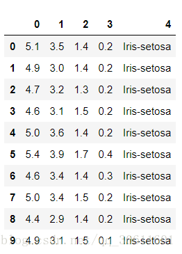
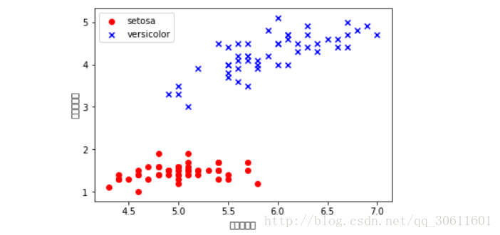
通过这些数字我们并不能明显看出什么关系，所以接下来，我们用matplotlib库画出其中两种花的两个变量的关系，我这里选取的是花瓣长度和花茎的长度

import matplotlib.pyplot as plt

y = df.loc[0:100, 4].values
y = np.where(y == 'Iris-setosa',-1,1)

x = df.loc[0:100,[0,2]].values

plt.scatter(x[:50,0],x[:50,1],color='red',marker='o',label='setosa')
plt.scatter(x[50:100,0],x[50:100,1],color='blue',marker='x',label='versicolor')
plt.xlabel('花瓣的长度')
plt.ylabel('花茎的长度')
plt.legend(loc = 'upper left')
plt.show()

通过图像我们可以很明显地看出，这两种花具有的特点

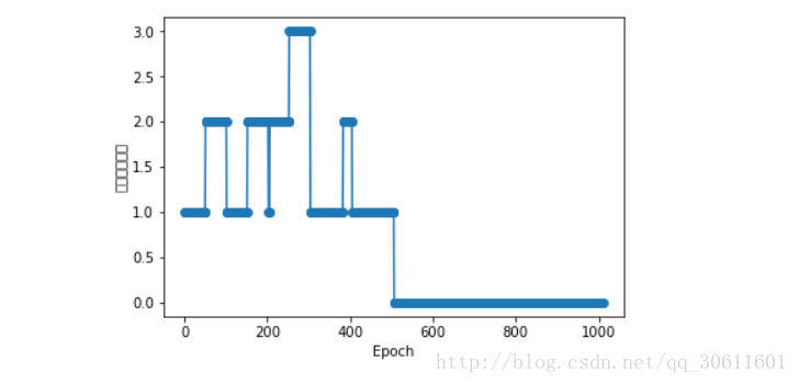
下面我们调用之前定义好的感知机模型，让它学习这些数据，然后我们同样画出感知机学习过程中的错误次数

ppn = Perception(eta=0.1, n_iter=10)
ppn.fit(x, y)
plt.plot(range(1,len(ppn.errors_) + 1),ppn.errors_, marker='o')
plt.xlabel('Epoch')
plt.ylabel('错误分类次数')
plt.show()

通过图中可以看出，在刚开始学习时，分类错误比较多，到后面就基本没有错误了

如果我们想要查看一下感知机学习出来的分离超平面可以定义如下一个绘图函数

from matplotlib.colors import ListedColormap
def plot_decision_regions(x, y, classifier, resolution = 0.02):
    marker = ('s', 'x', 'o', 'v')
    colors = ('red', 'blue', 'lightgreen', 'gray', 'cyan')
    cmap = ListedColormap(colors[:len(np.unique(y))])

    x1_min, x1_max = x[:,0].min() - 1, x[:,0].max()
    x2_min, x2_max = x[:,1].min() - 1, x[:,1].max()

    #print(x1_min, x1_max)
    #print(x2_min, x2_max)

    xx1, xx2 = np.meshgrid(np.arange(x1_min, x1_max, resolution),
                          np.arange(x2_min, x2_max, resolution))

    z = classifier.predict(np.array([xx1.ravel(), xx2.ravel()]).T)

    #print(xx1.ravel())
    #print(xx2.ravel())
    #print(z)

    z = z.reshape(xx1.shape)
    plt.contourf(xx1, xx2, z, alpha=0.4, cmap=cmap)
    plt.xlim(xx1.min(), xx1.max())
    plt.ylim(xx2.min(), xx2.max())

    for idx, cl in enumerate(np.unique(y)):
        plt.scatter(x=x[y==cl, 0],y=x[y==cl, 1], alpha=0.8, c=cmap(idx), 
                    marker=marker[idx], label=cl)

我们通过调用这个函数可以画出我们学习到的超平面

plot_decision_regions(x, y, ppn, resolution=0.02)
plt.xlabel('花瓣的长度')
plt.ylabel('花茎的长度')
plt.legend(loc = 'upper left')
plt.show()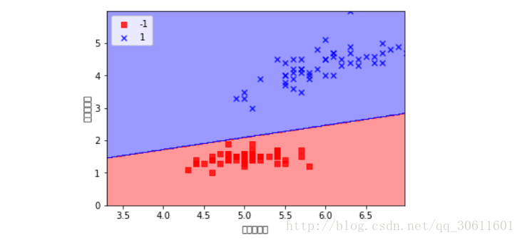

(PS: 在画图的时候忘记了中文的问题了。。。)