Implement Conjugate Priors in Python

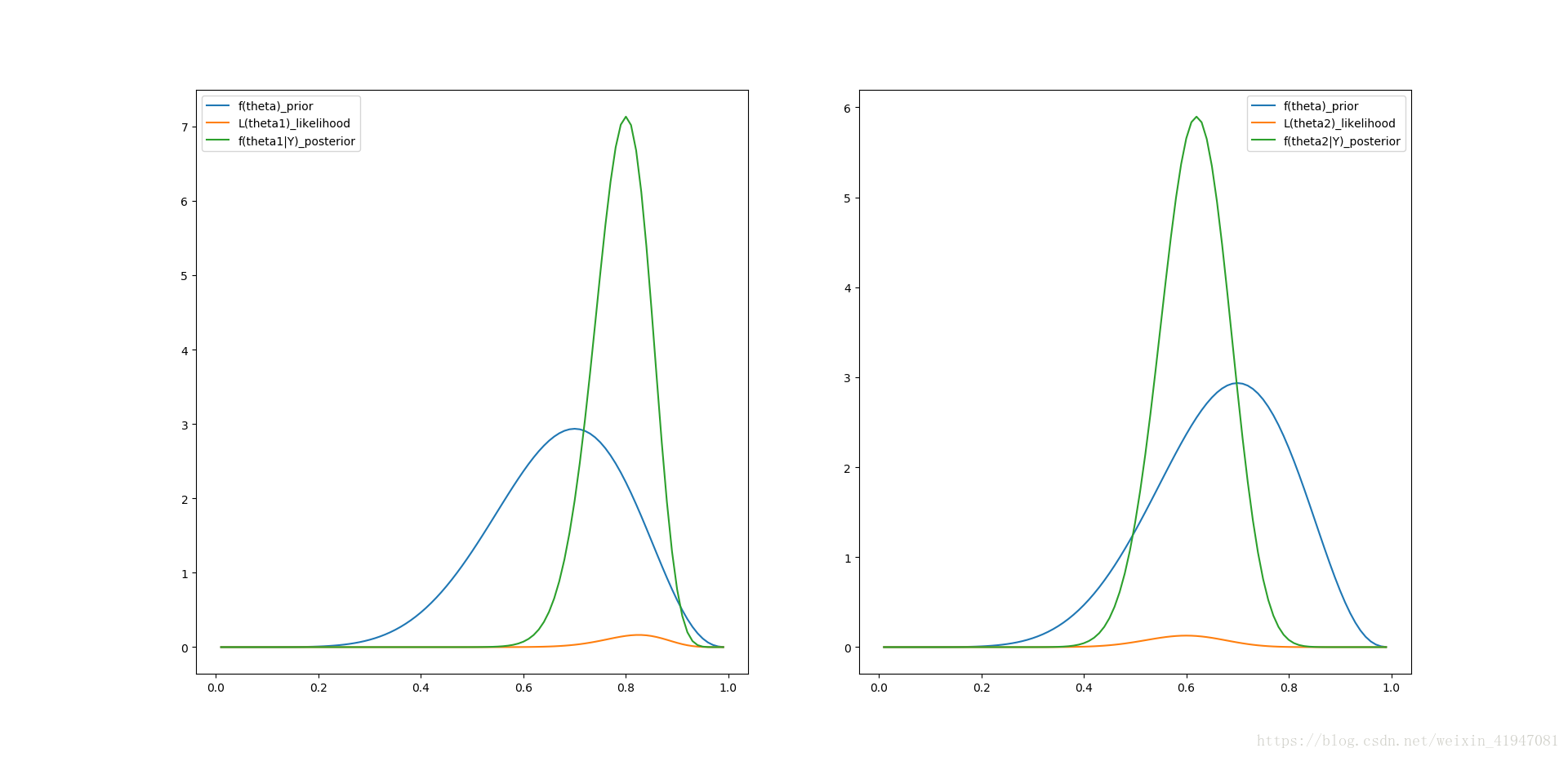
import numpy as np
from scipy.misc import factorial
import pandas as pd
import matplotlib.pyplot as plt
from scipy.stats import beta

# 让两个学生分别做40个选择题, 每个题有4种选择, 我们不知道这两个学生学得怎样,
# 不过可以认为他们的表现要比随机选择好.
# 两个学生的表现分别为theta1, theta2, 为beta分布
# 假设先验概率为alpha=8, beta=4, 就是说模拟测验, 两个学生都是10道题中作对的7道.
# 似然值为theta1学生这次测验中做对33道题, theta2学生只做对24道

def nCx(n,x):
    return factorial(n)/factorial(x)/factorial(n-x)
def binomdist(n, x, prob, accumulate=False):
    if not accumulate:
        return nCx(n,x) * (prob**x) * ( (1-prob)**(n-x) )
    if accumulate:
        answer = 0
        while 0 <= x:
            result = nCx(n,x) * (prob**x) * ( (1-prob)**(n-x) )
            answer += result
            x -= 1
        return answer
def beta_dist(alpha, beta, data):
    return factorial(alpha+beta-1)/factorial(alpha-1)/factorial(beta-1)*data**(alpha-1)*(1-data)**(beta-1)

df = pd.DataFrame()

alpha = 8
beta_ = 4
df['theta'] = np.arange(0.01,1,0.01)

# the prior - implement beta distribution
df['f(theta)_prior'] = beta_dist(alpha, beta_, df['theta'])
# likelihood for theta1
df['L(theta1)_likelihood'] = binomdist(40, 33, df['theta'])
# posterior for theta1
df['f(theta1|Y)_posterior'] = beta_dist(alpha+33, beta_+40-33, df['theta'])
# likelihood for theta2
df['L(theta2)_likelihood'] = binomdist(40, 24, df['theta'])
# posterior for theta2
df['f(theta2|Y)_posterior'] = beta_dist(alpha+24, beta_+40-24, df['theta'])

# prior P(theta>0.25)
a = sum(df['f(theta)_prior'][0:25])
b = sum(df['f(theta)_prior'][25:])
print('P(theta>0.25)', b/(a+b))

# The posterior prob. that theta1>theta2
theta1 = beta.rvs(alpha+33, beta_+40-33, size=1000)
theta2 = beta.rvs(alpha+24, beta_+40-24, size=1000)
print('Posterior prob. that theta1>theta2', sum(theta1 > theta2)/1000)

fig = plt.figure()
ax = fig.add_subplot(121)
ax.plot(df['theta'], df['f(theta)_prior'])
ax.plot(df['theta'], df['L(theta1)_likelihood'])
ax.plot(df['theta'], df['f(theta1|Y)_posterior'])
ax.legend()
ax1 = fig.add_subplot(122)
ax1.plot(df['theta'], df['f(theta)_prior'])
ax1.plot(df['theta'], df['L(theta2)_likelihood'])
ax1.plot(df['theta'], df['f(theta2|Y)_posterior'])
ax1.legend()
plt.show()