数字图像处理实验2

基本实验1

理解傅里叶谱和相位谱在视觉中的作用
程序代码：

clear;
RGB=imread('yangmi.bmp');%个人照片
I=rgb2gray(RGB); %x=rgb2gray(I);%彩色转灰度
figure;
subplot(221); imshow(I);
title('原始图像')
fi = fftshift(fft2(I));
fi_magn = abs(fi);
subplot(222); imshow(log(1+fi_magn),[]);
title('频谱图像');
fi_angl = angle(fi);
subplot(223);imshow(fi_angl,[]);
title('相位图像');
fi_shape = fi./fi_magn;
i_shape = ifft2(ifftshift(fi_shape));
subplot(224);
imshow(i_shape,[]);
title('形状图像')

实验结果：

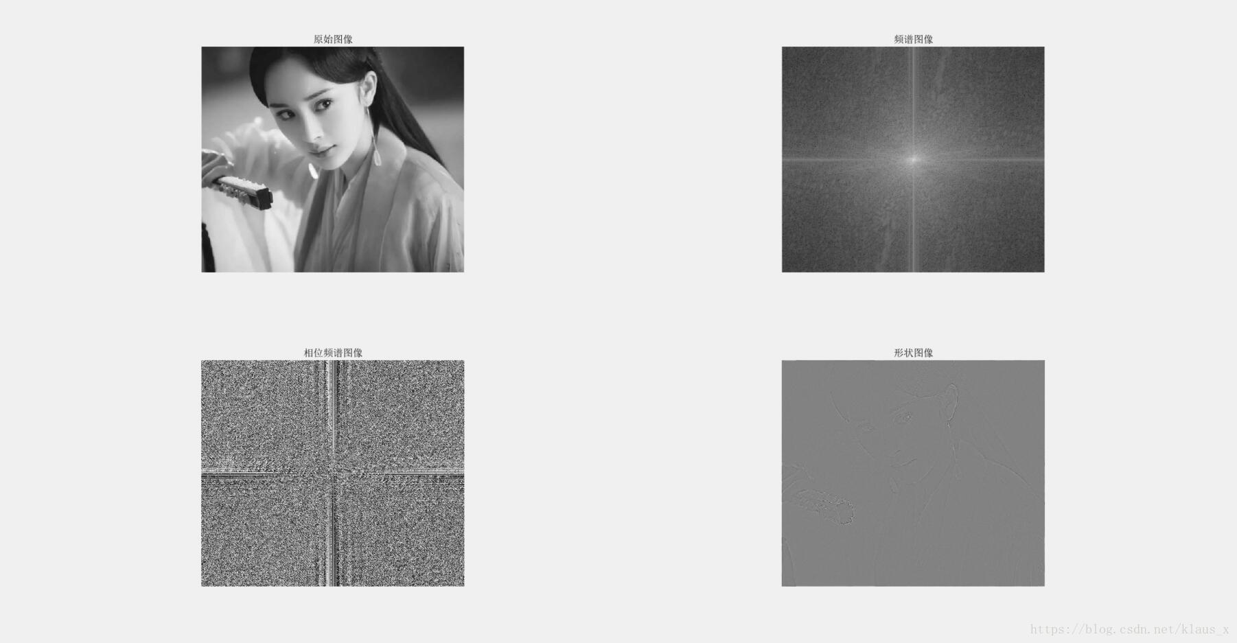
最后一张图，你们能看到杨幂的轮廓嘛？？？笑哭…笑哭

基本实验2：

对一副图像加入椒盐噪声后，实现2阶Butterworth低通滤波
程序代码如下：

clear;
RGB=imread('saturn.png');
I=rgb2gray(RGB);
subplot(221);imshow(I);title('原图')
I2 = imnoise(I,'salt & pepper');
subplot(222);imshow(I2);title('噪声图像');
[row,col]=size(I);
P = row*2;    Q = col*2;
f = zeros(P,Q);
f(1:row,1:col) = double(I2);
g = fft2(f);
g = fftshift(g);
result_ideal = zeros(P,Q);
result_buter = zeros(P,Q);
N = 2;%巴特沃斯滤波阶数
D0 = 50;%滤波半径
center_x = fix(P/2);
center_y = fix(Q/2);
tic;
for i=1:P
    for j=1:Q
        d_uv = sqrt((i-center_x)^2+(j-center_y)^2);
        h_ij = 1/(1+(d_uv/D0)^(2*N));
        result_buter(i,j) = h_ij*g(i,j);
        if(d_uv>D0)
            result_ideal(i,j)=0;
        else
            result_ideal(i,j)=g(i,j);
        end
    end
end
toc;
result_ideal = ifftshift(result_ideal);
result_buter = ifftshift(result_buter);
X1 = ifft2(result_buter);X2=uint8(real(X1));
result_B = X2(1:row,1:col);
subplot(223);imshow(result_B);
title('Butterworth滤波结果');
X3 = ifft2(result_ideal);X4=uint8(real(X3));
result_I = X4(1:row,1:col);
subplot(224);imshow(result_I);
title('理想滤波器滤波结果');

实验现象图

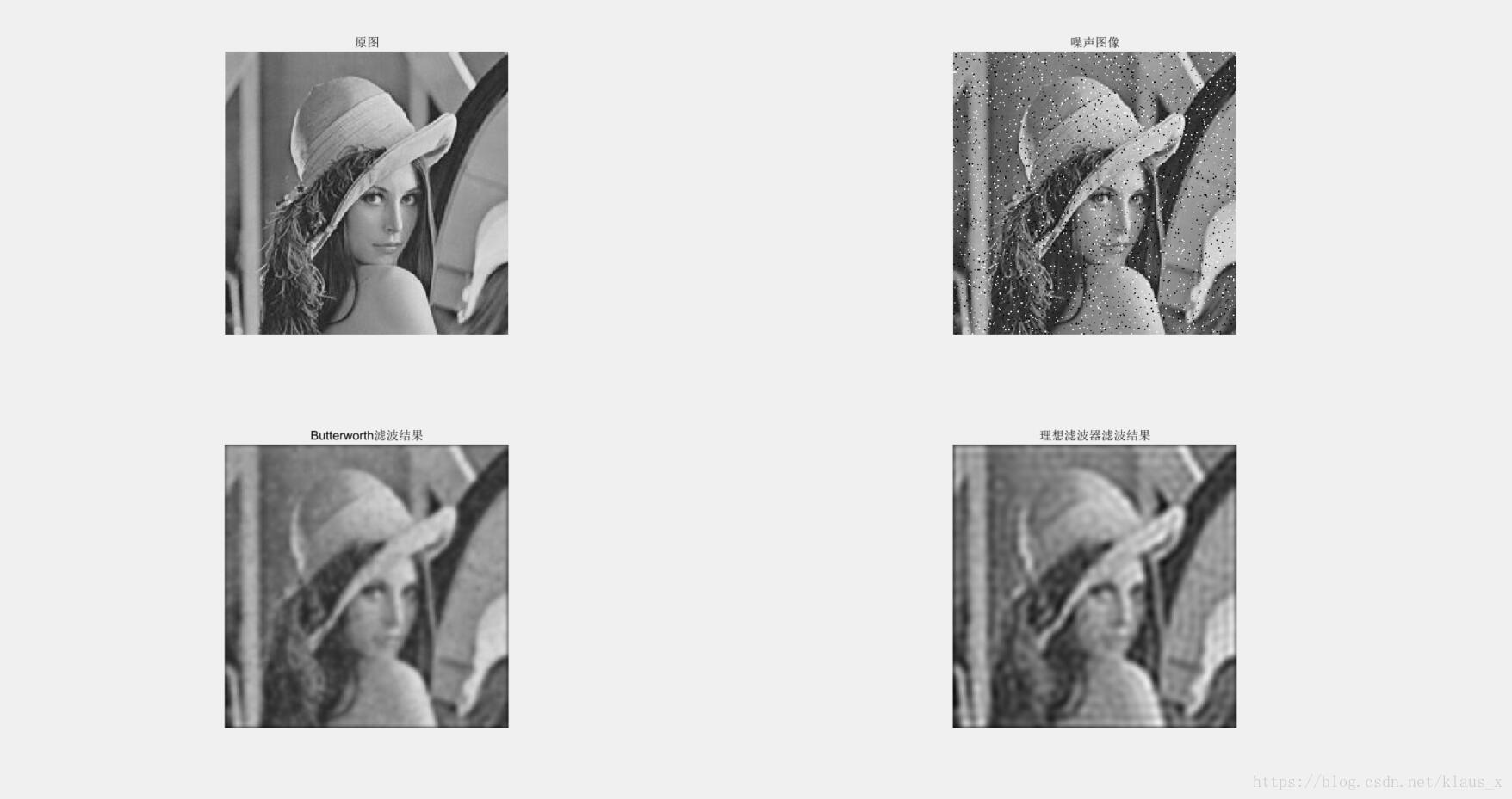
实验二涉及的数据比较多，博主建议给小一点的图像，也就是画质低一点的，上面这种图大概运行了大概运行了5秒左右（不能忍有木有！！！）；同时为了加快速度，也可以提前对迭代的数组赋值，减少运行时间。

基本实验3

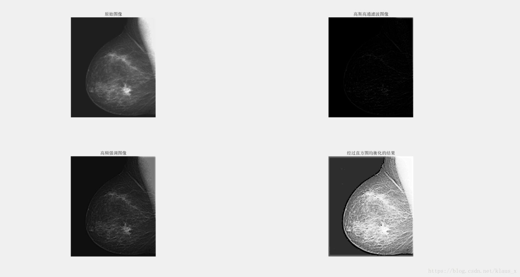
对一幅图像moon.tif实现高斯高频强调滤波
程序代码：

clear;
I = imread('chest_xray.tif');
figure;
subplot(221);imshow(I);title('原始图像');
%%
D0=40;
k1=0.5;
k2=0.75;
%%
[row,col]=size(I);
P = row*2;Q=col*2;
f = zeros(P,Q);
f(1:row,1:col)=double(I);
g=fft2(f);
g=fftshift(g);
center_x=fix(P/2);
center_y=fix(Q/2);
tic;

for i=1:P
    for j=1:Q
        duv2=(i-center_x)^2+(j-center_y)^2;
        h_uv=1-exp((-duv2/(2*D0*D0)));
        h_ij=k1+k2*h_uv;
        result_hp(i,j)=h_uv*g(i,j);
        result_hb(i,j)=h_ij*g(i,j);
    end
end

toc;
result_hp = uint8(real(ifft2(ifftshift(result_hp))));%进行反变换
result_hb = uint8(real(ifft2(ifftshift(result_hb))));%进行反变换
result_hp2=result_hp(1:row,1:col);
subplot(222);imshow(result_hp2);
title('高斯高通滤波图像')
result_hb2=result_hb(1:row,1:col);
subplot(223);imshow(result_hb2);
title('高频强调图像')；
resutlt_histeq=histeq(result_hb2);
subplot(224);
imshow(resutlt_histeq
);
title('经过直方图均衡化的结果')

实验现象结果

思考题

已知一同态滤波器的传输特性曲线如下图所示

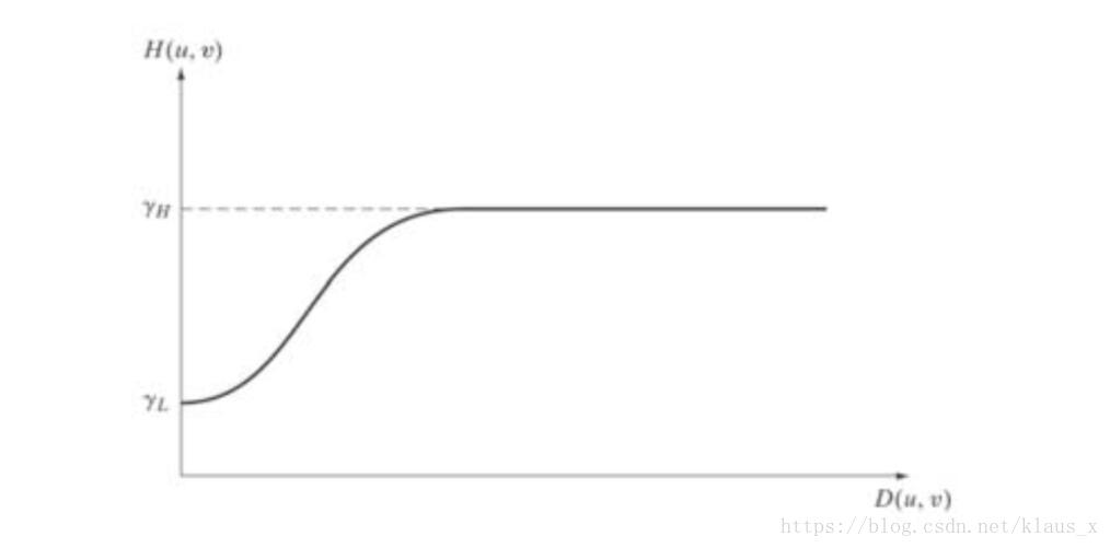
该滤波器的传递函数为：

H (u, v) = (γ_{H} - γ_{L}) [1 - e^{- c [\frac{D^{2} (u, v)}{{D_{0}}^{2}}]}] + γ_{L}

${\rm{H}}(u,v) = ({\gamma _H} - {\gamma _L})[1 - {e^{ - c[\frac{{{D^2}(u,v)}}{{{D_0}^2}}]}}] + {\gamma _L}$
设参数

γ_{H} = 2, γ_{L} = 0.25, c = 1, D_{0} = 80

${\gamma _H} = 2,{\gamma _L} = 0.25,c = 1,{D_0} = 80$
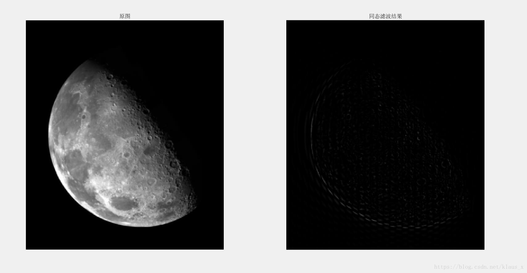
使用该同态滤波器对下图进行处理，编写M文件。
程序源码：

clear;
I = imread('moon.tif');
subplot(121);imshow(I);title('原图')
%%--------------------------
result_tt(1000,1000)=0;
rL=0.25;
rH=2;
c=1;
%%---------------------------
[row,col]=size(I);
P = row*2;    Q = col*2;
f = zeros(P,Q);
f(1:row,1:col)=double(I);
g = fft2(f);
g = fftshift(g);
D0 = 80;
center_x = fix(P/2);
center_y = fix(Q/2);
tic;
for i=1:P
    for j=1:Q
        d_uv = sqrt((i-center_x)^2+(j-center_y)^2);
        tmp=1-exp(c*(d_uv*d_uv/D0*D0));
        h_ij = (rH-rL)*tmp+rL;
        result_tt(i,j) = h_ij*g(i,j);
        if(d_uv>D0)
            result_tt(i,j)=g(i,j);
        else
            result_tt(i,j)=0;
        end
    end
end
toc;
result_tt = ifftshift(result_tt);
X1 = ifft2(result_tt);X2=uint8(real(X1));
result_B = X2(1:row,1:col);
subplot(122);imshow(result_B);
title('同态滤波结果');

实验结果：

如果需要下载我的文件的话，这里是程序源码和思考题的代码和文件夹的下载链接。
下载文件为压缩包形式。