- 查找轮廓的不同特征,例如面积,周长,重心,边界等
1.矩
图像的矩可以帮助我们计算图像的质心,面积等。
函数cv2.momen()会将计算得到的矩以一个字典的形式返回,
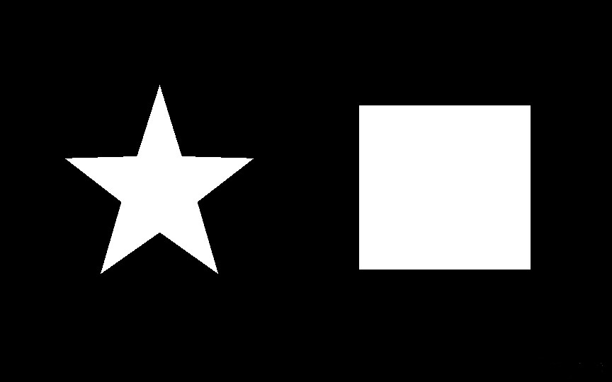
我们的测试图像如下:
例程如下:
# -*- coding:utf-8 -*-
import numpy as np
import cv2
from matplotlib import pyplot as plt
img = cv2.imread('8.jpg',0)
ret,thresh = cv2.threshold(img,127,255,0)
im,contours,hierarchy = cv2.findContours(thresh,cv2.RETR_TREE,cv2.CHAIN_APPROX_SIMPLE)
cnt = contours[0]
M = cv2.moments(cnt)
print(M)
#会返回一个字典
#计算重心
cx = int(M['m10']/M['m00'])
cy = int(M['m01']/M['m00'])
2.轮廓面积
轮廓面积可以用cv2.contourArea()计算得到,也可以使用矩,M['m00‘]
print(cv2.contourArea(cnt))
3.轮廓周长
也被称为弧长。可以使用函数cv2.arcLength()计算得到。这个函数的第二参数可以用来指定对象的形状是闭合的还是打开的(即曲线)
print(cv2.arcLength(cnt,True))#试了一下,如果强行赋予False,得到的周长会比用True短一些
4.轮廓近似
将轮廓形状近似到另外一种有更少点组成的轮廓形状,新轮廓的点的数目由我们设定的准确度来决定。使用的Douglas-Peucker算法在此不细讲了。
我们假设要在下图中找一个矩形
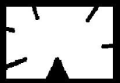
然而这个图凹凸不平,直接提取轮廓无法提取到一个完美的矩形。因此我们就可以使用这个函数来近似这个形状了。这个函数的第二个参数epsilon,是从原始轮廓到近似轮廓的最大距离,是一个准确度参数。因此对它的调整对最后的结果很重要。
例程如下:
# -*- coding:utf-8 -*-

import numpy as np
import  cv2
from matplotlib import pyplot as plt

im = cv2.imread('9.png')
img = cv2.cvtColor(im,cv2.COLOR_BGR2GRAY)#用这个方式转换的原因是最后输出时希望能看到彩色的的轮廓图
ret,thresh = cv2.threshold(img,127,255,0)

img,contours,hierarchy = cv2.findContours(thresh,1,2)
cnt = contours[0]

epsilon = 0.1*cv2.arcLength(cnt,True)
approx = cv2.approxPolyDP(cnt,epsilon,True)#这个和上面的True都是表示是闭曲线
#approx得到的仅仅是几个点集,需要将其连接起来

# cv2.drawContours(im,approx,-1,(0,0,255),3) 该函数只能画出几个点
cv2.polylines(im, [approx], True, (0, 255, 0), 2)#需要用这个函数才能画出轮廓,中间的True也是指示是否为闭曲线的

cv2.imshow('img',im)
cv2.waitKey(0)
最终效果如下:
指定为10%时: 指定为1%时:
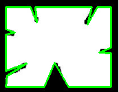
5.凸包
凸包与轮廓近似相似,有些时候他们给出的结果是一样的,但是本质上讲他们是不同的。函数cv2,convexHull()可以用来检测一个曲线是否具有凸性缺陷,并能纠正缺陷。一般来说,凸性曲线总是凸出来的,至少是频带。如果有地方凹进去了就被叫做凸性缺陷。如下图所示:
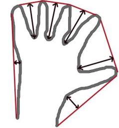
红色表示了他的凸包,而凸性缺陷被双箭头标出来了。
对于参数还有需要说明的地方:
hull = cv2.convexHull(points[],hull[],clockwise,retirnPoints)
- point是我们要传入的轮廓
- hull 输出,通常不需要
- clockwise 方向标志,如果设置为True,输出的凸包是顺时针方向的,否则为逆时针方向
- returnPoints 默认为True。它会返回凸包上点的坐标。如果设置为False,则会返回凸包点对应于原轮廓上的点坐标
实际操作中,不如需要获得上面的凸包,只需要:
hull = cv2.convexHull(cnt)
即可。但是如果你想获得凸性缺陷,需要把returnPoints设置为False。以上面的矩形为例,在获取他的轮廓cnt后,先把returnPoin设置为True查找凸包,会得到矩形的四个角点坐标。再将returnPoints设为False,将得到轮廓点的索引,即前面的四个坐标在原轮廓中的序列位置。
# -*- coding:utf-8 -*-
import numpy as np
import cv2
from matplotlib import pyplot as plt
im = cv2.imread('9.png')
img = cv2.cvtColor(im,cv2.COLOR_BGR2GRAY)#用这个方式转换的原因是最后输出时希望能看到彩色的的轮廓图
ret,thresh = cv2.threshold(img,127,255,0)
img,contours,hierarchy = cv2.findContours(thresh,1,2)
cnt = contours[0]
hull = cv2.convexHull(cnt,returnPoints=True)
print(hull)
# cv2.drawContours(im,hull,-1,(0,0,255),3) #该函数只能画出几个点
cv2.polylines(im, [hull], True, (0, 255, 0), 2)#需要用这个函数才能画出轮廓,中间的True也是指示是否为闭曲线的
cv2.imshow('img',im)
cv2.waitKey(0)
设置为True时得到的结果是
[[[161 126]]
[[ 8 126]]
[[ 8 10]]
[[161 10]]]
是矩形四个角点的坐标
设置为False后
[[113]
[ 60]
[ 0]
[126]]
表示的是上面四个点在cnt中的索引号,且不能画出凸包了
6.凸性检测
就是检测一个曲线是不是凸的,只能返回True和False
k = cv2.isContourConvex(cnt)
7.边界矩形
有两类边界矩形。
直边界矩形 一个直矩形(就是没有旋转的矩形)。它不会考虑对象是否旋转。所以边界矩形的面积不是最小的。可以使用函数cv2.boundingRect()查找得到的。
x,y,w,h = cv2.boundingRect(cnt)
img = cv2.rectangle(img,(x,y),(x+w,y+h),(0,255,0),2)
返回值中,(x,y)是矩阵左上角的坐标,(w,h)是举行的宽和高。
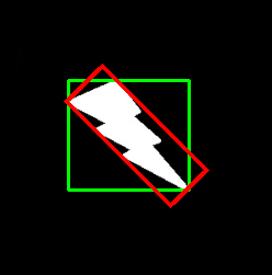
旋转边角矩形 这个边界矩形是面积最小的,因为他考虑了对象的旋转。用到的函数为cv2.minAreaRect()。返回的是一个Box2D结构,其中包含矩形左上角角点的坐标(x,y),以及矩形的宽和高(w,h),以及旋转角度。但是要绘制这个矩形需要矩形的4个角点。可以通过函数cv2.boxPoints()获得。
# -*- coding:utf-8 -*-

import numpy as np
import  cv2
from matplotlib import pyplot as plt

im = cv2.imread('10.png')
img = cv2.cvtColor(im,cv2.COLOR_BGR2GRAY)#用这个方式转换的原因是最后输出时希望能看到彩色的的轮廓图
ret,thresh = cv2.threshold(img,127,255,0)

img,contours,hierarchy = cv2.findContours(thresh,1,2)
cnt = contours[0]

#直边界矩形
x,y,w,h = cv2.boundingRect(cnt)
im = cv2.rectangle(im,(x,y),(x+w,y+h),(0,255,0),2)

#旋转边界矩形
s = cv2.minAreaRect(cnt)
a = cv2.boxPoints(s)
a = np.int0(a)#必须转换a的类型才能用polylines中画出,我也不知道为啥


cv2.polylines(im,[a],True,(0,0,255),3)

cv2.imshow('img',im)
cv2.waitKey(0)
最终效果如下:
8.最小外接圆
函数cv2.minEnclosingCircle() 可以帮我们找到一个对象的外切圆。它是所有能够包括对象的圆中面积中最小的一个。例程如下:
# -*- coding:utf-8 -*-
import numpy as np
import cv2
from matplotlib import pyplot as plt
im = cv2.imread('10.png')
img = cv2.cvtColor(im,cv2.COLOR_BGR2GRAY)#用这个方式转换的原因是最后输出时希望能看到彩色的的轮廓图
ret,thresh = cv2.threshold(img,127,255,0)
img,contours,hierarchy = cv2.findContours(thresh,1,2)
cnt = contours[0]
(x,y),radius = cv2.minEnclosingCircle(cnt)
center = (int(x),int(y))
radius = int(radius)
im = cv2.circle(im,center,radius,(0,255,0),2)
# cv2.polylines(im,[a],True,(0,0,255),3)
cv2.imshow('img',im)
cv2.waitKey(0)

9.椭圆拟合
使用cv2.fitEllipse()找椭圆,返回值就是旋转边界矩形的内切圆。用cv2.ellipse()画椭圆
# -*- coding:utf-8 -*-
import numpy as np
import cv2
from matplotlib import pyplot as plt
im = cv2.imread('10.png')
img = cv2.cvtColor(im,cv2.COLOR_BGR2GRAY)#用这个方式转换的原因是最后输出时希望能看到彩色的的轮廓图
ret,thresh = cv2.threshold(img,127,255,0)
img,contours,hierarchy = cv2.findContours(thresh,1,2)
cnt = contours[0]
ellise = cv2.fitEllipse(cnt)
im = cv2.ellipse(im,ellise,(0,255,0),2)
cv2.imshow('img',im)
cv2.waitKey(0)

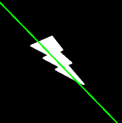
10.直线拟合
类似ゆ根据一组点拟合出一条直线,也可以根据 图像中的白色点拟合出一条直线,不过过程较为复杂
书上的例程如下:
# -*- coding:utf-8 -*-

import numpy as np
import  cv2
from matplotlib import pyplot as plt

im = cv2.imread('10.png')
img = cv2.cvtColor(im,cv2.COLOR_BGR2GRAY)#用这个方式转换的原因是最后输出时希望能看到彩色的的轮廓图
ret,thresh = cv2.threshold(img,127,255,0)

img,contours,hierarchy = cv2.findContours(thresh,1,2)
cnt = contours[0]

rows,cols = im.shape[:2]
#cv2.fitLine(points, distType, param, reps, aeps[, line ]) → line
#points – Input vector of 2D or 3D points, stored in std::vector<> or Mat.
#line – Output line parameters. In case of 2D fitting, it should be a vector of
#4 elements (likeVec4f) - (vx, vy, x0, y0), where (vx, vy) is a normalized
#vector collinear to the line and (x0, y0) is a point on the line. In case of
#3D fitting, it should be a vector of 6 elements (like Vec6f) - (vx, vy, vz,
#x0, y0, z0), where (vx, vy, vz) is a normalized vector collinear to the line
#and (x0, y0, z0) is a point on the line.
#distType – Distance used by the M-estimator
#distType=CV_DIST_L2
#ρ(r) = r2 /2 (the simplest and the fastest least-squares method)
#param – Numerical parameter ( C ) for some types of distances. If it is 0, an optimal value
#is chosen.
#reps – Sufficient accuracy for the radius (distance between the coordinate origin and the
#line).
#aeps – Sufficient accuracy for the angle. 0.01 would be a good default value for reps and
#aeps.
[vx,vy,x,y] = cv2.fitLine(cnt, cv2.DIST_L2,0,0.01,0.01)
lefty = int((-x*vy/vx) + y)
righty = int(((cols-x)*vy/vx)+y)
im = cv2.line(im,(cols-1,righty),(0,lefty),(0,255,0),2)

cv2.imshow('img',im)
cv2.waitKey(0)