深度学习中优化方法——momentum、Nesterov Momentum、AdaGrad、Adadelta、RMSprop、Adam

深度学习中优化方法

—momentum、Nesterov Momentum、AdaGrad、Adadelta、RMSprop、Adam—

我们通常使用梯度下降来求解神经网络的参数，关于梯度下降前面一篇博客已经很详细的介绍了（几种梯度下降方法对比）。我们在梯度下降时，为了加快收敛速度，通常使用一些优化方法，比如：momentum、RMSprop和Adam等。这篇博客主要介绍：

指数加权平均（Exponentially weighted average）
带偏差修正的指数加权平均（bias correction in exponentially weighted average）
momentum
Nesterov Momentum
Adagrad
Adadelta
RMSprop
Adam

在介绍这几种优化方法之前，必须先介绍下 指数加权平均（Exponentially weighted average） ，因为这个算法是接下来将要介绍的三个算法的重要组成部分。

一、 指数加权平均（Exponentially weighted average）

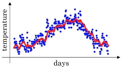
指数加权平均是处理时间序列的常用工具，下面用一个例子来引入指数加权平均的概念。下图是一个180天的气温图（图片来自ng Coursera deep learning 课）：

如果我们想找一条线去拟合这个数据，该怎么去做呢。我们知道某一天的气温其实和前几天（前一段时间）相关的，并不是一个独立的随机事件，比如夏天气温都会普遍偏高些，冬天气温普遍都会低一些。我们用 $[\theta_{1}、\theta_{2}、...、\theta_{n}]$ 表示第1，2，…，n天的气温，我们有：

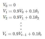
根据上面的公式我们能够画出这条线，如下图所示（图片来自ng deep learning课）：

下面来正式的看一下 指数加权平均（Exponentially weighted average） 的定义：

V_{t} = β V_{t - 1} + (1 - β) θ_{t}

$V_t = \beta V_{t-1} + (1- \beta) \theta_t$

可以认为 $V_t$ 近似是 $\frac{1}{1 - \beta}$ 天的平均气温，所以上面公式设置了 $\beta = 0.9$ ，当 $t > 10$ 时，则可以认为 $V_t$ 近似是它前10天的平均气温。
比如，按照上面的公式，我们计算 $V_{100}$ ，

\begin{array}{lcl} V_{100} & = & 0.1 θ_{100} + 0.9 V_{99} \\ = & 0.1 θ_{100} + 0.9 (0.9 V_{98} + 0.1 θ_{99}) = 0.1 θ_{100} + 0.9 * 0.1 θ_{99} + {0.9}^{2} V_{98} \\ = & 0.1 θ_{100} + 0.9 * 0.1 θ_{99} + {0.9}^{2} (0.9 V_{97} + 0.1 θ_{98}) = 0.1 θ_{100} + 0.9 * 0.1 θ_{99} + {0.9}^{2} * 0.1 θ_{98} + {0.9}^{3} V_{97} \\ = & 0.1 θ_{100} + 0.9 * 0.1 θ_{99} + {0.9}^{2} * 0.1 θ_{98} + {0.9}^{3} * 0.1 θ_{97} + {0.9}^{4} V_{96} \\ = & . . . . \\ = & 0.1 θ_{100} + 0.9 * 0.1 θ_{99} + {0.9}^{2} * 0.1 θ_{98} + {0.9}^{3} * 0.1 θ_{97} + . . . . + {0.9}^{99} * 0.1 θ_{1} + {0.9}^{100} V_{0} \end{array}

$\begin{array}{lcl} V_{100} &=& 0.1\theta_{100} + 0.9V_{99} \\ &=& 0.1\theta_{100} + 0.9(0.9V_{98} + 0.1\theta_{99}) = 0.1\theta_{100} + 0.9*0.1\theta_{99} + 0.9^2V_{98} \\ &=& 0.1\theta_{100} + 0.9*0.1\theta_{99} + 0.9^2(0.9V_{97} + 0.1\theta_{98}) = 0.1\theta_{100} + 0.9*0.1\theta_{99} + 0.9^2*0.1\theta_{98} + 0.9^3V_{97} \\ &=&0.1\theta_{100} + 0.9*0.1\theta_{99} + 0.9^2*0.1\theta_{98} + 0.9^3*0.1\theta_{97} + 0.9^4V_{96} \\ &=&....\\ &=&0.1\theta_{100} + 0.9*0.1\theta_{99} + 0.9^2*0.1\theta_{98} + 0.9^3*0.1\theta_{97} + ....+0.9^{99} * 0.1\theta_1 +0.9^{100}V_{0} \end{array}$

从上面的公式能够看出，实际上是个指数衰减函数。 $0.9^{10} \approx 0.35 \approx \frac{1}{e}$ ，所以这个就解释了上面的 $\frac{1}{1 - \beta}$ 。
（ps：关于这一点为什么要用0.35及 $\frac{1}{e}$ ，我是不太明白的，搜了下资料也没找到更好的资料，希望路过的有知道的大神，在下面评论交流。）
下面再看下 $\beta$ 取不同值时，曲线的拟合情况（图片来自ng deep learning课）：

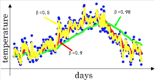
从上图能够看出：

当 $\beta$ 较大时（ $\beta = 0.98$ 相当于每一点前50天的平均气温），曲线波动相对较小更加平滑（绿色曲线），因为对很多天的气温做了平均处理，正因为如此，曲线还会右移。
同理，当 $\beta$ 较小时（ $\beta = 0.5$ 相当于每一点前2天的平均气温），曲线波动相对激烈，但是它可以更快的适应温度的变化。

下面直接看实现指数加权平均（Exponentially weighted average）的伪代码：

V0 = 0
repeat
{
    get next theta_t
    V_theta = beta * V_theta + (1 - beta)* theta_t
}

关于指数加权平均的优缺点：当 $\beta = 0.9$ 时，我们可以近似的认为当前的数值是过去10天的平均值，但是显然如果我们直接计算过去10天的平均值，要比用指数加权平均来的更加准确。但是如果直接计算过去10天的平均值，我们要存储过去10天的数值，而加权平均只要存储 $V_{t-1}$ 一个数值即可，而且只需要一行代码即可，所以在机器学习中用的很多。

二、带偏差修正的指数加权平均（bias correction in exponentially weighted average）

上一节中介绍了指数加权平均，用的公式是：

V_{t} = β V_{t - 1} + (1 - β θ_{t}

$V_t = \beta V_{t-1} + (1-\beta \theta_t$ )

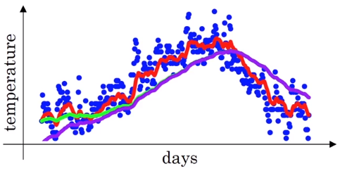
当我们令 $\beta = 0.98$ 时，我们想得到下图中的“绿线”，实际上我们得到的是下图中的“紫线”。对比这两条线，能够发现在“紫线”的起点相比“绿线”非常的低，举个例子，如果第一天的温度是40℃，按照上面的公式计算， $V_1 = 0.98 V_0 + (1-0.98)\theta_1 = 0.98*0 + 0.02 * 40 = 0.8$ ，按照这个公式预估第一天的温度是0.8℃，显然距离40℃，差距非常大。同样，继续计算，第二天的温度也没有很好的拟合，也就是说 指数加权平均 不能很好地拟合前几天的数据，因此需要 偏差修正，解决办法就是，再令 $V_t = \frac{V_t}{1 - \beta^t}$ 。因此， 带偏差修正的指数加权平均（bias correction in exponentially weighted average） 公式为：

\begin{array}{lcl} V_{t} & = & β V_{t - 1} + (1 - β θ_{t}) \\ V_{t} & = & \frac{V_{t}}{1 - β^{t}} \end{array}

$\begin{array}{lcl} V_t &=& \beta V_{t-1} + (1-\beta \theta_t )\\ V_t &=& \frac{V_t}{1 - \beta^t} \end{array}$

再来按照上述公式对前两天温度进行计算， $V_1 = \frac{V_1}{1 - \beta^1} = \frac{0.8}{1 -0.98} = 40$ ，能够发现温度没有偏差。并且当 $t \rightarrow \infty$ 时， $\beta^t \rightarrow 0$ ，这样在后期 $V_t$ 就和没有修正的指数加权平均一样了。

在机器学习中，多数的指数加权平均运算并不会使用偏差修正。因为大多数人更愿意在初始阶段，用一个捎带偏差的值进行运算。不过，如果在初试阶段就开始考虑偏差，指数加权移动均值仍处于预热阶段，偏差修正可以做出更好的估计。

介绍完上面的准备知识，下面正式进入正题。

三、动量（momentum）
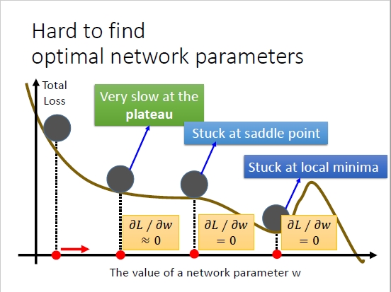
我们使用SGD（stochastic mini-batch gradient descent，深度学习中一般称之为SGD）训练参数时，有时候会下降的非常慢，并且可能会陷入到局部最小值中，如下图所示（图片来自李宏毅《一天搞懂深度学习》）。

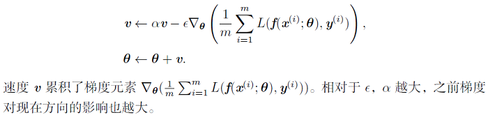
动量的引入就是为了加快学习过程，特别是对于高曲率、小但一致的梯度，或者噪声比较大的梯度能够很好的加快学习过程。动量的主要思想是积累了之前梯度指数级衰减的移动平均（前面的指数加权平均），下面用一个图来对比下，SGD和动量的区别：

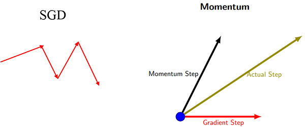
区别： SGD每次都会在当前位置上沿着负梯度方向更新（下降，沿着正梯度则为上升），并不考虑之前的方向梯度大小等等。而动量（moment）通过引入一个新的变量 $v$ 去积累之前的梯度（通过指数衰减平均得到），得到加速学习过程的目的。

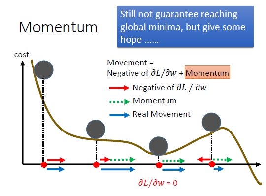
最直观的理解就是，若当前的梯度方向与累积的历史梯度方向一致，则当前的梯度会被加强，从而这一步下降的幅度更大。若当前的梯度方向与累积的梯度方向不一致，则会减弱当前下降的梯度幅度。

用一个图来形象的说明下上面这段话（图片来自李宏毅《一天搞懂深度学习》）：

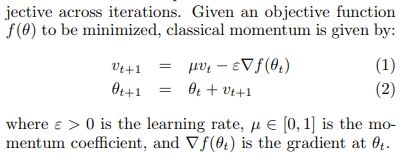
下面给出动量（momentum）的公式：

$\beta$ 的值越大，则之前的梯度对现在的方向影响越大。 $\beta$ 一般取值为0.5，0.9，0.99。ng推荐取值0.9。
这个公式是ng的在Coursera课上给出的。

关于这个公式目前主要有两种形式，*一种是原论文里的公式：（原论文：On the importance of initialization and momentum in deep learning）

使用这个公式的有：
1、 goodfellow和bengio的《deep learning》书：（8.3.2节 momentum）

2、 CS231N课（链接：http://cs231n.github.io/neural-networks-3/）：

# Momentum update
v = mu * v - learning_rate * dx # integrate velocity
x += v # integrate position

3、 keras：（链接：https://github.com/keras-team/keras/blob/master/keras/optimizers.py）

4、Intel的chainer框架，链接：https://github.com/chainer/chainer/blob/v4.0.0/chainer/optimizers/momentum_sgd.py

def update_core_cpu(self, param):
        grad = param.grad
        if grad is None:
            return
        v = self.state['v']
        if isinstance(v, intel64.mdarray):
            v.inplace_axpby(self.hyperparam.momentum, -
                            self.hyperparam.lr, grad)
            param.data += v
        else:
            v *= self.hyperparam.momentum
            v -= self.hyperparam.lr * grad
            param.data += v

*第二种是类似ng给的：
1、论文《An overview of gradient descent optimization algorithms》：

2、TensorFlow源码里的版本（链接：tensorflow/tensorflow/python/training/momentum.py）：

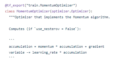
3、pytorch源码里的版本（链接：https://pytorch.org/docs/master/_modules/torch/optim/sgd.html#SGD）：

4、当时修hinton的nn课时，hinton给出的版本与TensorFlow这个是一样的，链接见我的博客：Hinton神经网络公开课编程题2–神经概率语言模型（NNLM）

这个版本是和ng在课上给出的版本是一致的，只不过会影响下learning_rate的取值。
综上，应该是哪个版本都可以。大家根据自己的喜好使用。

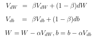
由于我个人更喜欢ng/TensorFlow/pytorch那个形式，下面无论是代码还是伪代码我都会统一用ng的版本，下面给出momentum的伪代码：

initialize VdW = 0, vdb = 0 //VdW维度与dW一致，Vdb维度与db一致
on iteration t:
    compute dW,db on current mini-batch
    VdW = beta*VdW + (1-beta)*dW
    Vdb = beta*Vdb + (1-beta)*db
    W = W - learning_rate * VdW
    b = b - learning_rate * Vdb

具体的代码实现为：

def initialize_velocity(parameters):
    """
    Initializes the velocity as a python dictionary with:
                - keys: "dW1", "db1", ..., "dWL", "dbL" 
                - values: numpy arrays of zeros of the same shape as the corresponding gradients/parameters.
    Arguments:
    parameters -- python dictionary containing your parameters.
                    parameters['W' + str(l)] = Wl
                    parameters['b' + str(l)] = bl

    Returns:
    v -- python dictionary containing the current velocity.
                    v['dW' + str(l)] = velocity of dWl
                    v['db' + str(l)] = velocity of dbl
    """
    L = len(parameters) // 2 # number of layers in the neural networks
    v = {}
    # Initialize velocity
    for l in range(L):
        v["dW" + str(l + 1)] = np.zeros(parameters["W" + str(l+1)].shape)
        v["db" + str(l + 1)] = np.zeros(parameters["b" + str(l+1)].shape)
    return v

def update_parameters_with_momentum(parameters, grads, v, beta, learning_rate):
    """
    Update parameters using Momentum
    Arguments:
    parameters -- python dictionary containing your parameters:
                    parameters['W' + str(l)] = Wl
                    parameters['b' + str(l)] = bl
    grads -- python dictionary containing your gradients for each parameters:
                    grads['dW' + str(l)] = dWl
                    grads['db' + str(l)] = dbl
    v -- python dictionary containing the current velocity:
                    v['dW' + str(l)] = ...
                    v['db' + str(l)] = ...
    beta -- the momentum hyperparameter, scalar
    learning_rate -- the learning rate, scalar
    Returns:
    parameters -- python dictionary containing your updated parameters 
    v -- python dictionary containing your updated velocities
    """
    L = len(parameters) // 2 # number of layers in the neural networks
    # Momentum update for each parameter
    for l in range(L):
        # compute velocities
        v["dW" + str(l + 1)] = beta * v["dW" + str(l + 1)] + (1 - beta) * grads['dW' + str(l + 1)]
        v["db" + str(l + 1)] = beta * v["db" + str(l + 1)] + (1 - beta) * grads['db' + str(l + 1)]
        # update parameters
        parameters["W" + str(l + 1)] = parameters["W" + str(l + 1)] - learning_rate * v["dW" + str(l + 1)]
        parameters["b" + str(l + 1)] = parameters["b" + str(l + 1)] - learning_rate * v["db" + str(l + 1)]
    return parameters, v

下面用sklearn中的breast_cancer数据集来对比下只用SGD（stochastic mini-batch gradient descent）和SGD with momentum：

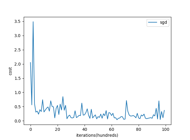
在测试集上的准确率是 0.91228。

在测试集上的准确率是 0.9210。

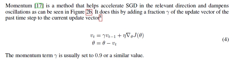
四、Nesterov Momentum
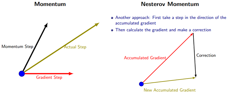
Nesterov Momentum是对Momentum的改进，可以理解为nesterov动量在标准动量方法中添加了一个校正因子。用一张图来形象的对比下momentum和nesterov momentum的区别（图片来自：http://ttic.uchicago.edu/~shubhendu/Pages/Files/Lecture6_pauses.pdf）：

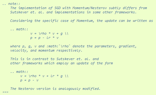
根据Sutskever et al （2013）的论文（On the importance of initialization and momentum in deep learning），nesterov momentum的公式如下：

goodfellow et al 的《deep learning》书中给的nesterov momentum算法：

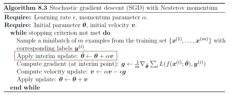
和momentum的唯一区别就是多了一步红色框框起来的步骤。

但是，我们仔细观察这个算法，你会发现一个很大的缺点，这个算法会导致运行速度巨慢无比，因为这个算法每次都要计算 $\nabla_\theta\sum_iL(f(x^{(i)};\theta + \alpha v),y^{(i)})，这个相当于又要把fp、bp走一遍。$ 这样就导致这个算法的运行速度比momentum要慢两倍，因此在实际实现过程中几乎没人直接用这个算法，而都是采用了变形版本。

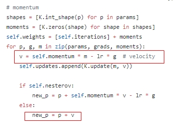
我们先来看看几个框架中nesterov momentum是怎么实现的：
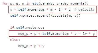
keras：https://github.com/keras-team/keras/blob/master/keras/optimizers.py#L146

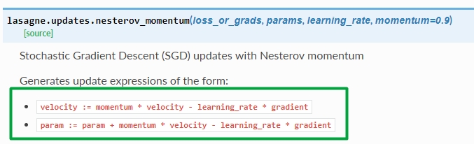
Lasagne：lasagne.updates.nesterov_momentum

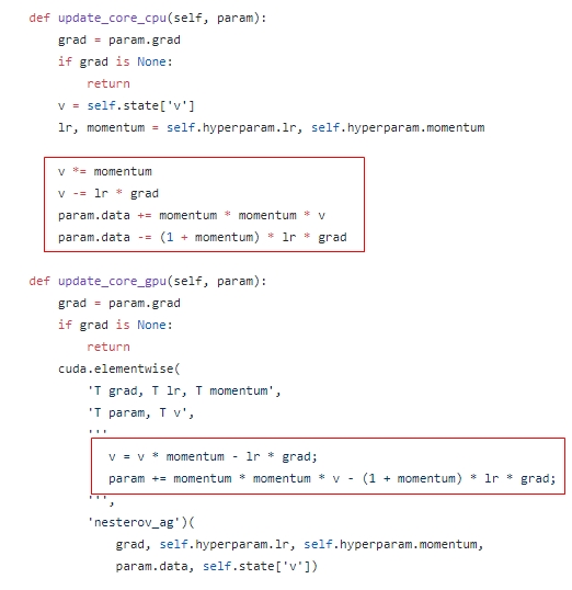
chainer：

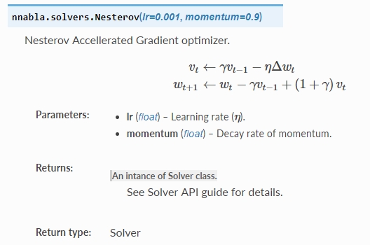
Neural Network Libraries：http://nnabla.readthedocs.io/en/latest/python/api/solver.html

CS231N：http://cs231n.github.io/neural-networks-3/

这些框架用的全是同一个公式：(提示：把上面的公式第一步代入第二步可以得到相同的公式： $w = w + \beta^2 V - (1 + \beta) \alpha*grad$ ）。我这里直接使用keras风格公式了，其中 $\beta$ 是动量参数， $\alpha$ 是学习率。

\begin{array}{lcl} V d W & = & β V d W - α d W \\ V d b & = & β V d b - α d b \\ W & = & W + β V d W - α d W \\ b & = & b + β V d b - α d b \end{array}

$\begin{array}{lcl} VdW &=& \beta VdW - \alpha dW \\\\ Vdb &=& \beta Vdb - \alpha db \\\\ W &=& W + \beta VdW - \alpha dW \\\\ b &=& b + \beta Vdb - \alpha db \end{array}$

这样写的高明之处在于，我们没必要去计算 $\nabla_\theta\sum_iL(f(x^{(i)};\theta + \alpha v),y^{(i)})$ 了，直接利用当前已求得的 $d\theta$ 去更新参数即可。这样就节省了一半的时间。

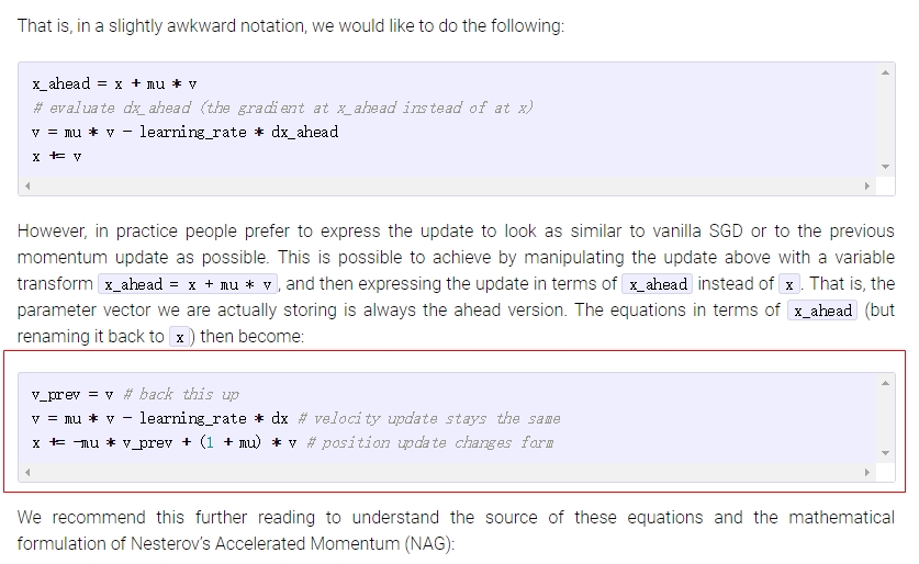
写到这里大家肯定会有一个疑问，为什么这个公式就是正确的，这和原公式（论文中和《deep learning》书中提到的公式）形式明显不一样。下面我来推导证明这两个公式为什么是一样的：
先看原始公式：

\begin{array}{lcl} V_{t + 1} & = & β V_{t} - α \nabla_{θ_{t}} L (θ_{t} + β V_{t}) \\ θ_{t + 1} & = & θ_{t} + V_{t + 1} \end{array}

$\begin{array}{lcl} V_{t+1} &=& \beta V_t - \alpha \nabla_{\theta_t}L(\theta_t + \beta V_t) \\\\ \theta_{t+1} &=& \theta_{t} + V_{t+1} \end{array}$

下面是推导过程（参考资料：1、cs231n中Nesterov Momentum段中However, in practice people prefer to express the update….这段话 2、9987 用Theano实现Nesterov momentum的正确姿势）：
首先令 ${\theta _{t}}' = \theta _{t} + \beta V_t$ ，则 $V_{t+1} = \beta V_t - \alpha \nabla_{\theta_t}L({\theta _{t}}')$
则：

\begin{array}{lcl} {θ_{t + 1}}^{'} & = & θ_{t + 1} + β V_{t + 1} \\ = & θ_{t} + V_{t + 1} + β V_{t + 1} \\ = & θ_{t} + (1 + β) V_{t + 1} \\ = & {θ_{t}}^{'} - β V_{t} + (1 + β) [β V_{t} - α \nabla_{{θ_{t}}^{'}} L ({θ_{t}}^{'})] \\ = & {θ_{t}}^{'} + β^{2} V_{t} - (1 + β) α \nabla_{{θ_{t}}^{'}} L ({θ_{t}}^{'}) \end{array}

$\begin{array}{lcl} {\theta _{t+1}}' &=& \theta _{t+1} + \beta V_{t+1} \\\\ &=& \theta_t + V_{t+1} + \beta V_{t+1}\\\\ &=& \theta_t + (1+ \beta)V_{t+1}\\\\ &=& {\theta _{t}}' - \beta V_t + (1+\beta)[\beta V_t - \alpha \nabla_{{\theta _{t}}'}L({\theta _{t}}')] \\\\ &=& {\theta _{t}}' + \beta^{2}V_t - (1+\beta) \alpha \nabla_{{\theta _{t}}'}L({\theta _{t}}') \end{array}$

下面替换回来，令 $\theta _{t} = {\theta _{t}}'$ ，则上述公式为： $\theta _{t+1} = \theta _{t}+ \beta^{2}V_t - (1+\beta) \alpha \nabla_{\theta _{t}}L(\theta _{t})$

下面是实现的代码（初始化和momentum一样就不贴出初始化的代码了）：

#nesterov momentum
def update_parameters_with_nesterov_momentum(parameters, grads, v, beta, learning_rate):
    """
    Update parameters using Momentum
    Arguments:
    parameters -- python dictionary containing your parameters:
                    parameters['W' + str(l)] = Wl
                    parameters['b' + str(l)] = bl
    grads -- python dictionary containing your gradients for each parameters:
                    grads['dW' + str(l)] = dWl
                    grads['db' + str(l)] = dbl
    v -- python dictionary containing the current velocity:
                    v['dW' + str(l)] = ...
                    v['db' + str(l)] = ...
    beta -- the momentum hyperparameter, scalar
    learning_rate -- the learning rate, scalar

    Returns:
    parameters -- python dictionary containing your updated parameters
    v -- python dictionary containing your updated velocities

    '''
    VdW = beta * VdW - learning_rate * dW
    Vdb = beta * Vdb - learning_rate * db
    W = W + beta * VdW - learning_rate * dW
    b = b + beta * Vdb - learning_rate * db
    '''
    """

    L = len(parameters) // 2  # number of layers in the neural networks

    # Momentum update for each parameter
    for l in range(L):
        # compute velocities
        v["dW" + str(l + 1)] = beta * v["dW" + str(l + 1)] - learning_rate * grads['dW' + str(l + 1)]
        v["db" + str(l + 1)] = beta * v["db" + str(l + 1)] - learning_rate * grads['db' + str(l + 1)]
        # update parameters
        parameters["W" + str(l + 1)] += beta * v["dW" + str(l + 1)]- learning_rate * grads['dW' + str(l + 1)]
        parameters["b" + str(l + 1)] += beta * v["db" + str(l + 1)] - learning_rate * grads["db" + str(l + 1)]

    return parameters

论文《An overview of gradient descent optimization algorithms》中写道：This anticipatory update prevents us from going too fast and results in increased responsiveness, which has significantly increased the performance of RNNs on a number of tasks

五、AdaGrad（Adaptive Gradient）
通常，我们在每一次更新参数时，对于所有的参数使用相同的学习率。而AdaGrad算法的思想是：每一次更新参数时（一次迭代），不同的参数使用不同的学习率。AdaGrad 的公式为：

\begin{array}{lcl} G_{t} & = & G_{t - 1} + g_{t}^{2} \\ θ_{t + 1} & = & θ_{t} - \frac{α}{\sqrt{G_{t}} + ε} \cdot g_{t} \end{array}

$\begin{array}{lcl} G_t &=& G_{t-1} + g^2_t \\\\ \theta_{t+1} &=& \theta_{t} - \frac{\alpha }{\sqrt{G_t } + \varepsilon}\cdot g_t \end{array}$

从公式中我们能够发现：
优点：对于梯度较大的参数， $G_t$ 相对较大，则 $\frac{\alpha }{\sqrt{G_t }+ \varepsilon }$ 较小，意味着学习率会变得较小。而对于梯度较小的参数，则效果相反。这样就可以使得参数在平缓的地方下降的稍微快些，不至于徘徊不前。
缺点：由于是累积梯度的平方，到后面 $G_t$ 累积的比较大，会导致梯度 $\frac{\alpha }{\sqrt{G_t }+ \varepsilon } \rightarrow 0$ ，导致梯度消失。

关于AdaGrad，goodfellow和bengio的《deep learning》书中对此的描述是：在凸优化中，AdaGrad算法具有一些令人满意的理论性质。但是，在实际使用中已经发现，对于训练深度神经网络模型而言，从训练开始时累积梯度平方会导致学习率过早过量的减少。AdaGrad算法在某些深度学习模型上效果不错，但不是全部。

具体到实现，对于 $iteration \ t，compute \ on \ current \ mini-batch：$

\begin{array}{lcl} G_{w} & = & G_{w} + (d W)^{2} \\ W & = & W - \frac{α}{\sqrt{G_{w}} + ε} \cdot d W \\ G_{b} & = & G_{b} + (d b)^{2} \\ b & = & b - \frac{α}{\sqrt{G_{b}} + ε} \cdot d b \end{array}

$\begin{array}{lcl} G_w &=& G_{w} + (dW)^2 \\ W &=& W - \frac{\alpha }{\sqrt{G_w }+ \varepsilon }\cdot dW \\\\ G_b &=& G_{b} + (db)^2 \\ b &=& b - \frac{\alpha }{\sqrt{G_b}+ \varepsilon }\cdot db \end{array}$

其中 $\varepsilon$ 一般默认取 $10^{-7}$ （《deep learning》书和mxnet），学习率 $\alpha$ 一般取值为 $0.01$ （论文：《An overview of gradient descent optimization algorithms》）。
代码实现：

#AdaGrad initialization
def initialize_adagrad(parameters):
    """
    Initializes the velocity as a python dictionary with:
                - keys: "dW1", "db1", ..., "dWL", "dbL"
                - values: numpy arrays of zeros of the same shape as the corresponding gradients/parameters.
    Arguments:
    parameters -- python dictionary containing your parameters.
                    parameters['W' + str(l)] = Wl
                    parameters['b' + str(l)] = bl

    Returns:
    Gt -- python dictionary containing sum of the squares of the gradients up to step t.
                    G['dW' + str(l)] = sum of the squares of the gradients up to dwl
                    G['db' + str(l)] = sum of the squares of the gradients up to db1
    """
    L = len(parameters) // 2  # number of layers in the neural networks
    G = {}
    # Initialize velocity
    for l in range(L):
        G["dW" + str(l + 1)] = np.zeros(parameters["W" + str(l + 1)].shape)
        G["db" + str(l + 1)] = np.zeros(parameters["b" + str(l + 1)].shape)
    return G

#AdaGrad
def update_parameters_with_adagrad(parameters, grads, G, learning_rate, epsilon = 1e-7):
    """
    Update parameters using Momentum
    Arguments:
    parameters -- python dictionary containing your parameters:
                    parameters['W' + str(l)] = Wl
                    parameters['b' + str(l)] = bl
    grads -- python dictionary containing your gradients for each parameters:
                    grads['dW' + str(l)] = dWl
                    grads['db' + str(l)] = dbl
    G -- python dictionary containing the current velocity:
                    G['dW' + str(l)] = ...
                    G['db' + str(l)] = ...
    learning_rate -- the learning rate, scalar
    epsilon -- hyperparameter preventing division by zero in adagrad updates

    Returns:
    parameters -- python dictionary containing your updated parameters

    '''
    GW += (dW)^2
    W -= learning_rate/(sqrt(GW) + epsilon)*dW
    Gb += (db)^2
    b -= learning_rate/(sqrt(Gb)+ epsilon)*db
    '''
    """

    L = len(parameters) // 2  # number of layers in the neural networks

    # Momentum update for each parameter
    for l in range(L):
        # compute velocities
        G["dW" + str(l + 1)] += grads['dW' + str(l + 1)]**2
        G["db" + str(l + 1)] += grads['db' + str(l + 1)]**2
        # update parameters
        parameters["W" + str(l + 1)] -= learning_rate / (np.sqrt(G["dW" + str(l + 1)]) + epsilon) * grads['dW' + str(l + 1)]
        parameters["b" + str(l + 1)] -= learning_rate / (np.sqrt(G["db" + str(l + 1)]) + epsilon) * grads['db' + str(l + 1)]

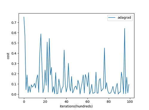
    return parameters

简单的跑了下，准确率是0.9386，代价函数随着迭代次数的变化如下图：

六、Adadelta
Adadelta是对Adagrad的改进，主要是为了克服Adagrad的两个缺点（摘自Adadelta论文《AdaDelta: An Adaptive Learning Rate Method》）：

the continual decay of learning rates throughout training
the need for a manually selected global learning rate

为了解决第一个问题，Adadelta只累积过去 $w$ 窗口大小的梯度，其实就是利用前面讲过的指数加权平均，公式如下：

E [g^{2}]_{t} = ρ E [g^{2}]_{t - 1} + (1 - ρ) g_{t}^{2}

$E[g^2]_t = \rho E[g^2]_{t-1} + (1 - \rho)g^2_t$

根据前面讲到的指数加权平均，比如当 $\rho = 0.9$ 时，则相当于累积前10个梯度。
为了解决第二个问题，Adadelta最终的公式不需要学习率 $\alpha$ 。Adadelta的具体算法如下所示（来自论文《AdaDelta: An Adaptive Learning Rate Method》）：

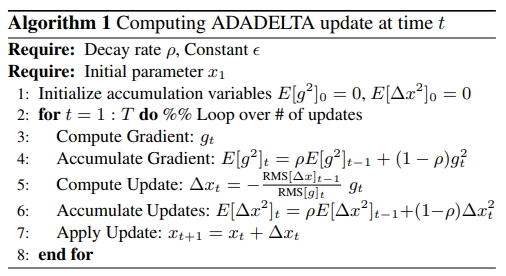
可以看到adadelta算法不在需要学习率，p.s：看了keras和Lasagne框架的adadelta源码，它们依然使用了学习率，不知道为什么。。。而chainer框架则没有使用。
按照我们的习惯重新写下上述公式：

\begin{array}{lcl} S_{d w} & = & ρ S_{d w} + (1 - ρ) (d W)^{2} \\ S_{d b} & = & ρ S_{d b} + (1 - ρ) (d b)^{2} \\ V_{d w} & = & \sqrt{\frac{\nabla_{w} + ε}{S_{d w} + ε}} \cdot d W \\ V_{d b} & = & \sqrt{\frac{\nabla_{b} + ε}{S_{d b} + ε}} \cdot d b \\ W & = & W - V_{d w} \\ b & = & b - V_{d b} \\ \nabla_{w} & = & ρ \nabla_{w} + (1 - ρ) (V_{d w})^{2} \\ \nabla_{b} & = & ρ \nabla_{b} + (1 - ρ) (V_{d b})^{2} \end{array}

$\begin{array}{lcl} S_{dw} &=& \rho S_{dw} + (1 - \rho)(dW)^2 \\ S_{db} &=& \rho S_{db} + (1 - \rho)(db)^2 \\\\ V_{dw} &=& \sqrt{\frac{\nabla_w + \varepsilon}{S_{dw} + \varepsilon }}\cdot dW \\ V_{db} &=& \sqrt{\frac{\nabla_b + \varepsilon}{S_{db} + \varepsilon }}\cdot db \\\\ W &=& W - V_{dw}\\ b &=& b - V_{db}\\\\ \nabla_w &=& \rho \nabla_w + (1 - \rho)(V_{dw})^2 \\ \nabla_b &=& \rho \nabla_b + (1 - \rho)(V_{db})^2 \\\\ \end{array}$

其中 $\varepsilon$ 是为了防止分母为0，通常取 $1e^-6$ 。
下面是代码实现：

#initialize_adadelta
def initialize_adadelta(parameters):
    """
    Initializes s and delta as two python dictionaries with:
                - keys: "dW1", "db1", ..., "dWL", "dbL"
                - values: numpy arrays of zeros of the same shape as the corresponding gradients/parameters.

    Arguments:
    parameters -- python dictionary containing your parameters.
                    parameters["W" + str(l)] = Wl
                    parameters["b" + str(l)] = bl

    Returns:
    s -- python dictionary that will contain the exponentially weighted average of the squared gradient of dw
                    s["dW" + str(l)] = ...
                    s["db" + str(l)] = ...
    v -- python dictionary that will contain the RMS
                v["dW" + str(l)] = ...
                v["db" + str(l)] = ...
    delta -- python dictionary that will contain the exponentially weighted average of the squared gradient of delta_w
                    delta["dW" + str(l)] = ...
                    delta["db" + str(l)] = ...

    """

    L = len(parameters) // 2  # number of layers in the neural networks
    s = {}
    v = {}
    delta = {}
    # Initialize s, v, delta. Input: "parameters". Outputs: "s, v, delta".
    for l in range(L):
        s["dW" + str(l + 1)] = np.zeros(parameters["W" + str(l + 1)].shape)
        s["db" + str(l + 1)] = np.zeros(parameters["b" + str(l + 1)].shape)
        v["dW" + str(l + 1)] = np.zeros(parameters["W" + str(l + 1)].shape)
        v["db" + str(l + 1)] = np.zeros(parameters["b" + str(l + 1)].shape)
        delta["dW" + str(l + 1)] = np.zeros(parameters["W" + str(l + 1)].shape)
        delta["db" + str(l + 1)] = np.zeros(parameters["b" + str(l + 1)].shape)

    return s, v, delta

#adadelta
def update_parameters_with_adadelta(parameters, grads, rho, s, v, delta, epsilon = 1e-6):
    """
    Update parameters using Momentum
    Arguments:
    parameters -- python dictionary containing your parameters:
                    parameters['W' + str(l)] = Wl
                    parameters['b' + str(l)] = bl
    grads -- python dictionary containing your gradients for each parameters:
                    grads['dW' + str(l)] = dWl
                    grads['db' + str(l)] = dbl
    rho -- decay constant similar to that used in the momentum method, scalar
    s -- python dictionary containing the current velocity:
                    s['dW' + str(l)] = ...
                    s['db' + str(l)] = ...
    delta -- python dictionary containing the current RMS:
                    delta['dW' + str(l)] = ...
                    delta['db' + str(l)] = ...

    epsilon -- hyperparameter preventing division by zero in adagrad updates

    Returns:
    parameters -- python dictionary containing your updated parameters

    '''
    Sdw = rho*Sdw + (1 - rho)*(dW)^2
    Sdb = rho*Sdb + (1 - rho)*(db)^2
    Vdw = sqrt((delta_w + epsilon) / (Sdw + epsilon))*dW
    Vdb = sqrt((delta_b + epsilon) / (Sdb + epsilon))*dW
    W -= Vdw
    b -= Vdb
    delta_w = rho*delta_w + (1 - rho)*(Vdw)^2
    delta_b = rho*delta_b + (1 - rho)*(Vdb)^2
    '''
    """

    L = len(parameters) // 2  # number of layers in the neural networks
    # adadelta update for each parameter
    for l in range(L):
        # compute s
        s["dW" + str(l + 1)] = rho * s["dW" + str(l + 1)] + (1 - rho)*grads['dW' + str(l + 1)]**2
        s["db" + str(l + 1)] = rho * s["db" + str(l + 1)] + (1 - rho)*grads['db' + str(l + 1)]**2
        #compute RMS
        v["dW" + str(l + 1)] = np.sqrt((delta["dW" + str(l + 1)] + epsilon) / (s["dW" + str(l + 1)] + epsilon)) * grads['dW' + str(l + 1)]
        v["db" + str(l + 1)] = np.sqrt((delta["db" + str(l + 1)] + epsilon) / (s["db" + str(l + 1)] + epsilon)) * grads['db' + str(l + 1)]
        # update parameters
        parameters["W" + str(l + 1)] -= v["dW" + str(l + 1)]
        parameters["b" + str(l + 1)] -= v["db" + str(l + 1)]
        #compute delta
        delta["dW" + str(l + 1)] = rho * delta["dW" + str(l + 1)] + (1 - rho) * v["dW" + str(l + 1)] ** 2
        delta["db" + str(l + 1)] = rho * delta["db" + str(l + 1)] + (1 - rho) * v["db" + str(l + 1)] ** 2

    return parameters

七、RMSprop（root mean square prop）
RMSprop是hinton老爷子在Coursera的《Neural Networks for Machine Learning》lecture6中提出的，这个方法并没有写成论文发表（不由的感叹老爷子的强大。。以前在Coursera上修过这门课，个人感觉不算简单）。同样的，RMSprop也是对Adagrad的扩展，以在非凸的情况下效果更好。和Adadelta一样，RMSprop使用指数加权平均（指数衰减平均）只保留过去给定窗口大小的梯度，使其能够在找到凸碗状结构后快速收敛。直接来看下RMSprop的算法（来自lan goodfellow 《deep learning》）：

在实际使用过程中，RMSprop已被证明是一种有效且实用的深度神经网络优化算法。目前它是深度学习人员经常采用的优化算法之一。keras文档中关于RMSprop写到：This optimizer is usually a good choice for recurrent neural networks.

按照我们的习惯，重写下公式：

\begin{array}{lcl} S_{d w} & = & β S_{d w} + (1 - ρ) (d W)^{2} \\ S_{d b} & = & ρ S_{d b} + (1 - ρ) (d b)^{2} \\ W & = & W - α \frac{d W}{\sqrt{S_{d W} + ε}} \\ b & = & b - α \frac{d b}{\sqrt{S_{d b} + ε}} \end{array}

$\begin{array}{lcl} S_{dw} &=& \beta S_{dw} + (1 - \rho)(dW)^2 \\ S_{db} &=& \rho S_{db} + (1 - \rho)(db)^2 \\\\ W &=& W - \alpha\frac{dW}{\sqrt{S_{dW} + \varepsilon}}\\ b &=& b - \alpha\frac{db}{\sqrt{S_{db} + \varepsilon}} \end{array}$

同样 $\varepsilon$ 是为了防止分母为0，默认值设为 $1e^{-6}$ 。 $\beta$ 默认值设为 $0.9$ ，学习率 $\alpha$ 默认值设为 $0.001$ 。
具体实现为：

#RMSprop
def update_parameters_with_rmsprop(parameters, grads, s, beta = 0.9, learning_rate = 0.01, epsilon = 1e-6):
    """
    Update parameters using Momentum
    Arguments:
    parameters -- python dictionary containing your parameters:
                    parameters['W' + str(l)] = Wl
                    parameters['b' + str(l)] = bl
    grads -- python dictionary containing your gradients for each parameters:
                    grads['dW' + str(l)] = dWl
                    grads['db' + str(l)] = dbl
    s -- python dictionary containing the current velocity:
                    v['dW' + str(l)] = ...
                    v['db' + str(l)] = ...
    beta -- the momentum hyperparameter, scalar
    learning_rate -- the learning rate, scalar

    Returns:
    parameters -- python dictionary containing your updated parameters
    '''
    SdW = beta * SdW + (1-beta) * (dW)^2
    sdb = beta * Sdb + (1-beta) * (db)^2
    W = W - learning_rate * dW/sqrt(SdW + epsilon)
    b = b - learning_rate * db/sqrt(Sdb + epsilon)
    '''
    """
    L = len(parameters) // 2  # number of layers in the neural networks
    # rmsprop update for each parameter
    for l in range(L):
        # compute velocities
        s["dW" + str(l + 1)] = beta * s["dW" + str(l + 1)] + (1 - beta) * grads['dW' + str(l + 1)]**2
        s["db" + str(l + 1)] = beta * s["db" + str(l + 1)] + (1 - beta) * grads['db' + str(l + 1)]**2
        # update parameters
        parameters["W" + str(l + 1)] = parameters["W" + str(l + 1)] - learning_rate * grads['dW' + str(l + 1)] / np.sqrt(s["dW" + str(l + 1)] + epsilon)
        parameters["b" + str(l + 1)] = parameters["b" + str(l + 1)] - learning_rate * grads['db' + str(l + 1)] / np.sqrt(s["db" + str(l + 1)] + epsilon)

    return parameters

八、Adam（Adaptive Moment Estimation）
Adam实际上是把momentum和RMSprop结合起来的一种算法，算法流程是（摘自adam论文）：

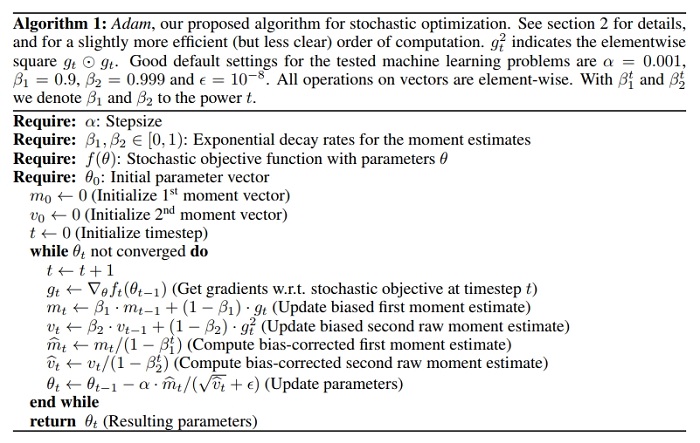
同样，简洁的写一下公式：

其中，几个参数推荐的默认值分别为： $\alpha = 0.001，\beta_1 = 0.9，\beta_2 = 0.999，\varepsilon = 10^{-8}$ 。 $t$ 是迭代次数，每个mini-batch后，都要进行 t += 1。

下面是具体的代码：

#initialize adam
def initialize_adam(parameters):
    """
    Initializes v and s as two python dictionaries with:
                - keys: "dW1", "db1", ..., "dWL", "dbL"
                - values: numpy arrays of zeros of the same shape as the corresponding gradients/parameters.
    Arguments:
    parameters -- python dictionary containing your parameters.
                    parameters["W" + str(l)] = Wl
                    parameters["b" + str(l)] = bl
    Returns:
    v -- python dictionary that will contain the exponentially weighted average of the gradient.
                    v["dW" + str(l)] = ...
                    v["db" + str(l)] = ...
    s -- python dictionary that will contain the exponentially weighted average of the squared gradient.
                    s["dW" + str(l)] = ...
                    s["db" + str(l)] = ...

    """
    L = len(parameters) // 2  # number of layers in the neural networks
    v = {}
    s = {}
    # Initialize v, s. Input: "parameters". Outputs: "v, s".
    for l in range(L):
        v["dW" + str(l + 1)] = np.zeros(parameters["W" + str(l + 1)].shape)
        v["db" + str(l + 1)] = np.zeros(parameters["b" + str(l + 1)].shape)
        s["dW" + str(l + 1)] = np.zeros(parameters["W" + str(l + 1)].shape)
        s["db" + str(l + 1)] = np.zeros(parameters["b" + str(l + 1)].shape)

    return v, s

#adam
def update_parameters_with_adam(parameters, grads, v, s, t, learning_rate=0.01, beta1=0.9, beta2=0.999, epsilon=1e-8):
    """
    Update parameters using Adam

    Arguments:
    parameters -- python dictionary containing your parameters:
                    parameters['W' + str(l)] = Wl
                    parameters['b' + str(l)] = bl
    grads -- python dictionary containing your gradients for each parameters:
                    grads['dW' + str(l)] = dWl
                    grads['db' + str(l)] = dbl
    v -- Adam variable, moving average of the first gradient, python dictionary
    s -- Adam variable, moving average of the squared gradient, python dictionary
    learning_rate -- the learning rate, scalar.
    beta1 -- Exponential decay hyperparameter for the first moment estimates
    beta2 -- Exponential decay hyperparameter for the second moment estimates
    epsilon -- hyperparameter preventing division by zero in Adam updates

    Returns:
    parameters -- python dictionary containing your updated parameters
    """

    L = len(parameters) // 2  # number of layers in the neural networks
    v_corrected = {}  # Initializing first moment estimate, python dictionary
    s_corrected = {}  # Initializing second moment estimate, python dictionary

    # Perform Adam update on all parameters
    for l in range(L):
        # Moving average of the gradients. Inputs: "v, grads, beta1". Output: "v".
        v["dW" + str(l + 1)] = beta1 * v["dW" + str(l + 1)] + (1 - beta1) * grads['dW' + str(l + 1)]
        v["db" + str(l + 1)] = beta1 * v["db" + str(l + 1)] + (1 - beta1) * grads['db' + str(l + 1)]
        # Compute bias-corrected first moment estimate. Inputs: "v, beta1, t". Output: "v_corrected".
        v_corrected["dW" + str(l + 1)] = v["dW" + str(l + 1)] / (1 - np.power(beta1, t))
        v_corrected["db" + str(l + 1)] = v["db" + str(l + 1)] / (1 - np.power(beta1, t))
        # Moving average of the squared gradients. Inputs: "s, grads, beta2". Output: "s".
        s["dW" + str(l + 1)] = beta2 * s["dW" + str(l + 1)] + (1 - beta2) * np.power(grads['dW' + str(l + 1)], 2)
        s["db" + str(l + 1)] = beta2 * s["db" + str(l + 1)] + (1 - beta2) * np.power(grads['db' + str(l + 1)], 2)
        # Compute bias-corrected second raw moment estimate. Inputs: "s, beta2, t". Output: "s_corrected".
        s_corrected["dW" + str(l + 1)] = s["dW" + str(l + 1)] / (1 - np.power(beta2, t))
        s_corrected["db" + str(l + 1)] = s["db" + str(l + 1)] / (1 - np.power(beta2, t))
        # Update parameters. Inputs: "parameters, learning_rate, v_corrected, s_corrected, epsilon". Output: "parameters".
        parameters["W" + str(l + 1)] = parameters["W" + str(l + 1)] - learning_rate * v_corrected["dW" + str(l + 1)] / np.sqrt(s_corrected["dW" + str(l + 1)] + epsilon)
        parameters["b" + str(l + 1)] = parameters["b" + str(l + 1)] - learning_rate * v_corrected["db" + str(l + 1)] / np.sqrt(s_corrected["db" + str(l + 1)] + epsilon)

    return parameters

实践表明，Adam算法在很多种不同的神经网络结构中都是非常有效的。

八、该如何选择优化算法
介绍了这么多算法，那么我们到底该选择哪种算法呢？目前还没有一个共识，schaul et al 在大量学习任务上比较了许多优化算法，结果表明，RMSprop，Adadelta和Adam表现的相当鲁棒，不分伯仲。Kingma et al表明带偏差修正的Adam算法稍微好于RMSprop。总之，Adam算法是一个相当好的选择，通常会得到比较好的效果。

下面是论文《An overview of gradient descent optimization algorithms》对各种优化算法的总结：

In summary, RMSprop is an extension of Adagrad that deals with its radically diminishing learning rates. It is identical to Adadelta, except that Adadelta uses the RMS of parameter updates in the numerator update rule. Adam, finally, adds bias-correction and momentum to RMSprop. Insofar, RMSprop, Adadelta, and Adam are very similar algorithms that do well in similar circumstances. Kingma et al. [10] show that its bias-correction helps Adam slightly outperform RMSprop towards the end of optimization as gradients become sparser. Insofar, Adam might be the best overall choice

完整的代码已放到github上：deep_neural_network_with_optimizers.py

参考文献：
[1]:Andrew Ng 《Improving Deep Neural Networks: Hyperparameter tuning, Regularization and Optimization》
[2]:Shubhendu Trivedi et al. CMSC 35246 : Deep Learning 《Optimization for Deep Neural Networks》
[3]:Timothy Dozat. Incorporating Nesterov Momentum into Adam
[4]:Diederik P. Kingma et al. ADAM: A Method For Stochastic Optimization, ICLR2015
[5]:Ilya Sutskever et al On the importance of initialization and momentum in deep learning, JMLR2013
[6]: lan goodfellow et al. 《deep learning》
[7]: 王赟 Maigo. 用Theano实现Nesterov momentum的正确姿势
[8]: TensorFlow
[9]: keras
[10]: pytorch
[11]: Neural Network Libraries
[12]: Orange3-Recommendation
[13]: Lasagne
[14]: Fei-Fei Li et al. 《CS231n Convolutional Neural Networks for Visual Recognition》
[15]: Geoffrey Hinton.《Neural Networks for Machine Learning》
[16]: Sebastian Ruder. An overview of gradient descent optimization algorithms
[17]: Matthew Zeiler. AdaDelta: An Adaptive Learning Rate Method
[18]: Diederik P. Kingma et al. ADAM: A METHOD FOR STOCHASTIC OPTIMIZATION, ICLR2015
[19]: Tom Schaul et al. Unit Tests for Stochastic Optimization, ICLR2014