一个简单的DEMO:实现手写数字图片的识别
单向LSTM
利用的数据集是tensorflow提供的一个手写数字数据集。该数据集是一个包含55000张28*28的数据集。
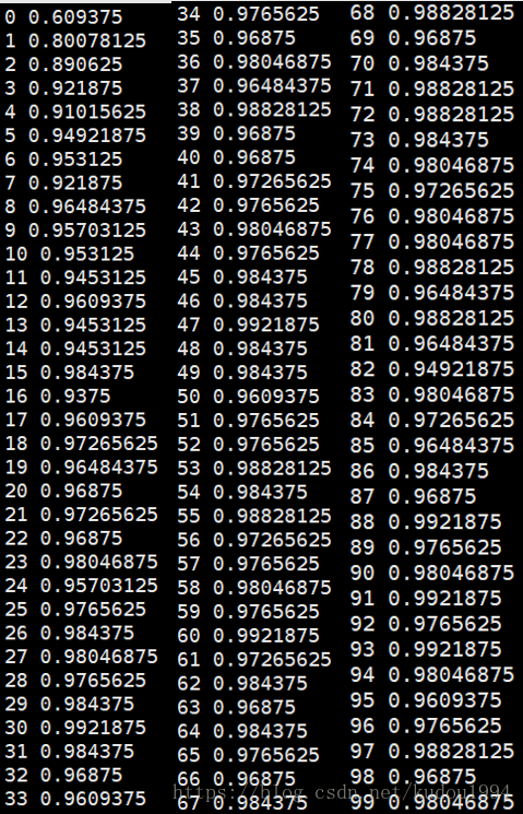
训练100次
识别准确率还不是很稳定,但是从第17次开始就趋于相对稳定的状态了。
# -*- coding: utf-8 -*-
import tensorflow as tf
from tensorflow.contrib import rnn

import numpy as np
#import input_data
from tensorflow.examples.tutorials.mnist import input_data #####
mnist = input_data.read_data_sets('MNIST_data', one_hot=True) #####

# configuration
#                        O * W + b -> 10 labels for each image, O[? 28], W[28 10], B[10]
#                       ^ (O: output 28 vec from 28 vec input)
#                       |
#      +-+  +-+       +--+
#      |1|->|2|-> ... |28| time_step_size = 28
#      +-+  +-+       +--+
#       ^    ^    ...  ^
#       |    |         |
# img1:[28] [28]  ... [28]
# img2:[28] [28]  ... [28]
# img3:[28] [28]  ... [28]
# ...
# img128 or img256 (batch_size or test_size 256)
#      each input size = input_vec_size=lstm_size=28

# configuration variables
input_vec_size = lstm_size = 28 # 输入向量的维度
time_step_size = 28 # 循环层长度

batch_size = 128
test_size = 256

def init_weights(shape):
    return tf.Variable(tf.random_normal(shape, stddev=0.01))


def model(X, W, B, lstm_size):
    # X, input shape: (batch_size, time_step_size, input_vec_size)
    # XT shape: (time_step_size, batch_size, input_vec_size)
    #对这一步操作还不是太理解,为什么需要将第一行和第二行置换
    XT = tf.transpose(X, [1, 0, 2])  # permute time_step_size and batch_size,[28, 128, 28]


    # XR shape: (time_step_size * batch_size, input_vec_size)
    XR = tf.reshape(XT, [-1, lstm_size]) # each row has input for each lstm cell (lstm_size=input_vec_size)

    # Each array shape: (batch_size, input_vec_size)
    X_split = tf.split(XR, time_step_size, 0) # split them to time_step_size (28 arrays),shape = [(128, 28),(128, 28)...]


    # Make lstm with lstm_size (each input vector size). num_units=lstm_size; forget_bias=1.0
    lstm = rnn.BasicLSTMCell(lstm_size, forget_bias=1.0, state_is_tuple=True)

    # Get lstm cell output, time_step_size (28) arrays with lstm_size output: (batch_size, lstm_size)
    # rnn..static_rnn()的输出对应于每一个timestep,如果只关心最后一步的输出,取outputs[-1]即可
    outputs, _states = rnn.static_rnn(lstm, X_split, dtype=tf.float32)  # 时间序列上每个Cell的输出:[... shape=(128, 28)..]

    # tanh activation
    # Get the last output
    return tf.matmul(outputs[-1], W) + B, lstm.state_size # State size to initialize the state

mnist = input_data.read_data_sets("MNIST_data/", one_hot=True) # 读取数据

# mnist.train.images是一个55000 * 784维的矩阵, mnist.train.labels是一个55000 * 10维的矩阵
#训练集包含55000张图片,每张图片为28*28维矩阵
#训练集标签同样对应55000,10表示存在10个标签
trX, trY, teX, teY = mnist.train.images, mnist.train.labels, mnist.test.images, mnist.test.labels

# 将每张图用一个28x28的矩阵表示,(55000,28,28,1)
#-1表示该数未知,根据后面28*28,将trx分成55000个28*28的矩阵,每个表示一张图片。

trX = trX.reshape(-1, 28, 28)
teX = teX.reshape(-1, 28, 28)

X = tf.placeholder("float", [None, 28, 28])
Y = tf.placeholder("float", [None, 10])

# get lstm_size and output 10 labels
#生成一个初始随机值
W = init_weights([lstm_size, 10])  # 输出层权重矩阵28×10
B = init_weights([10])  # 输出层bais

#
py_x, state_size = model(X, W, B, lstm_size)

cost = tf.reduce_mean(tf.nn.softmax_cross_entropy_with_logits(logits=py_x, labels=Y))
train_op = tf.train.RMSPropOptimizer(0.001, 0.9).minimize(cost)
#返回每一行的最大值
predict_op = tf.argmax(py_x, 1)

#tf.ConfigProto,一般是在创建session时对session进行配置
session_conf = tf.ConfigProto()
session_conf.gpu_options.allow_growth = True#允许gpu在使用的过程中慢慢增加。

# Launch the graph in a session
with tf.Session(config=session_conf) as sess:
    # you need to initialize all variables
    tf.global_variables_initializer().run()
    for i in range(100):
        #从训练集中每段选择一个batch训练,batch_size= end-start
        for start, end in zip(range(0, len(trX), batch_size), range(batch_size, len(trX)+1, batch_size)):
            sess.run(train_op, feed_dict={X: trX[start:end], Y: trY[start:end]})
            #X (128,28,28)
        s=len(teX)
        test_indices = np.arange(len(teX))  # Get A Test Batch
        np.random.shuffle(test_indices)
        test_indices = test_indices[0:test_size]

        print(i, np.mean(np.argmax(teY[test_indices], axis=1) ==
                         sess.run(predict_op, feed_dict={X: teX[test_indices]})))
结果:
双向LSTM
利用的数据集是tensorflow提供的一个手写数字数据集。该数据集是一个包含55000张28*28的数据集。
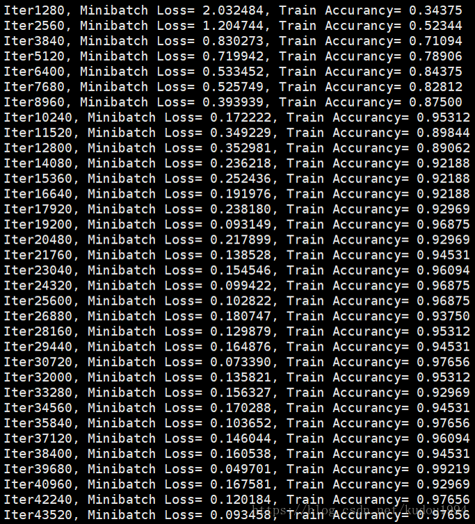
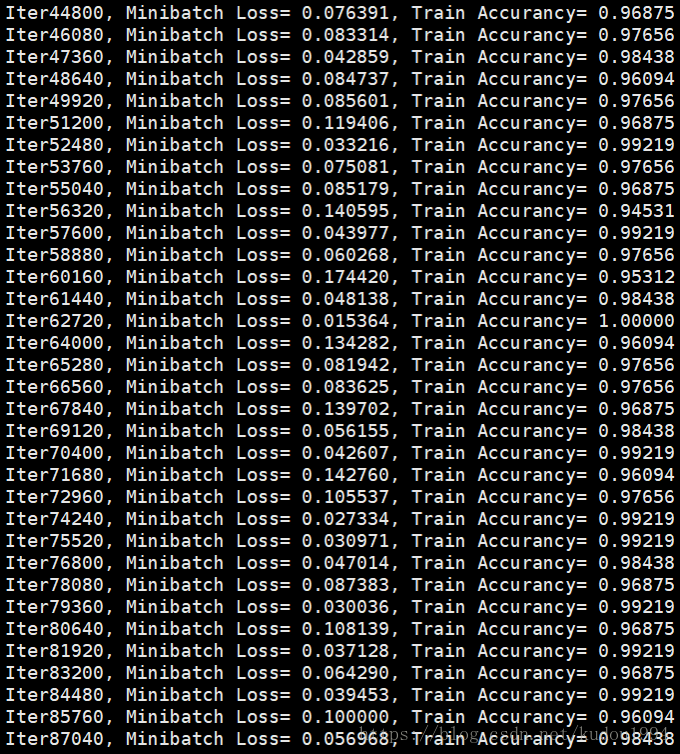
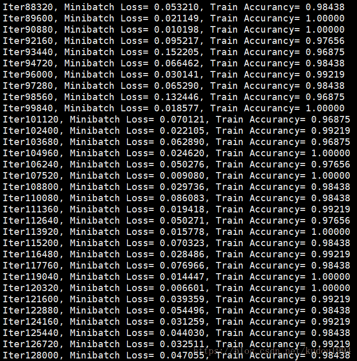
训练300次
可以看到使用双向LSTM要训练更多次才能趋于相对稳定,但是经过100次训练后,准确率明显比单向LSTM要高,稳定性要好。
#coding:utf-8
import tensorflow as tf
import numpy as np
from tensorflow.examples.tutorials.mnist import input_data
mnist = input_data.read_data_sets("/tmp/data", one_hot=True)


learning_rate = 0.01
max_samples = 400000
display_size = 10
batch_size = 128

#实际上图的像素列数,每一行作为一个输入,输入到网络中。
n_input = 28
#LSTM cell的展开宽度,对于图像来说,也是图像的行数
#也就是图像按时间步展开是按照行来展开的。
n_step = 28
#LSTM cell个数
n_hidden = 256
n_class = 10


x = tf.placeholder(tf.float32, shape=[None, n_step, n_input])
y = tf.placeholder(tf.float32, shape =[None, n_class])

#这里的参数只是最后的全连接层的参数,调用BasicLSTMCell这个op,参数已经包在内部了,不需要再定义。
Weight = tf.Variable(tf.random_normal([2 * n_hidden, n_class]))   #参数共享力度比cnn还大
bias = tf.Variable(tf.random_normal([n_class]))


def BiRNN(x, weights, biases):
    #[1, 0, 2]只做第阶和第二阶的转置
    x = tf.transpose(x, [1, 0, 2])
    #把转置后的矩阵reshape成n_input列,行数不固定的矩阵。
    #对一个batch的数据来说,实际上有bacth_size*n_step行。
    x = tf.reshape(x, [-1, n_input])  #-1,表示样本数量不固定
    #拆分成n_step组
    x = tf.split(x, n_step)
    #调用现成的BasicLSTMCell,建立两条完全一样,又独立的LSTM结构
    lstm_qx = tf.contrib.rnn.BasicLSTMCell(n_hidden, forget_bias = 1.0)
    lstm_hx = tf.contrib.rnn.BasicLSTMCell(n_hidden, forget_bias = 1.0)
    #两个完全一样的LSTM结构输入到static_bidrectional_rnn中,由这个op来管理双向计算过程。
    outputs, _, _ = tf.contrib.rnn.static_bidirectional_rnn(lstm_qx, lstm_hx, x, dtype = tf.float32)
    #最后来一个全连接层分类预测
    return tf.matmul(outputs[-1], weights) + biases


pred = BiRNN(x, Weight, bias)
#计算损失、优化、精度(老套路)
cost = tf.reduce_mean(tf.nn.softmax_cross_entropy_with_logits(logits = pred, labels = y))
optimizer = tf.train.AdamOptimizer(learning_rate = learning_rate).minimize(cost)
correct_pred = tf.equal(tf.argmax(pred, 1), tf.argmax(y, 1))
accurancy = tf.reduce_mean(tf.cast(correct_pred, tf.float32))

init = tf.global_variables_initializer()

#run图过程。
with tf.Session() as sess:
    sess.run(init)
    step = 1
    while step * batch_size < max_samples:
        batch_x, batch_y = mnist.train.next_batch(batch_size)
        batch_x = batch_x.reshape((batch_size, n_step, n_input))
        sess.run(optimizer, feed_dict = {x:batch_x, y:batch_y})
        if step % display_size == 0:
            acc = sess.run(accurancy, feed_dict={x:batch_x, y:batch_y})
            loss = sess.run(cost, feed_dict = {x:batch_x, y:batch_y})
            print 'Iter' + str(step*batch_size) + ', Minibatch Loss= %.6f'%(loss) + ', Train Accurancy= %.5f'%(acc)

        step += 1
    print "Optimizer Finished!"


    test_len = 10000
    test_data = mnist.test.images[:test_len].reshape(-1, n_step, n_input)
    test_label = mnist.test.labels[:test_len]
    print 'Testing Accurancy:%.5f'%(sess.run(accurancy, feed_dict={x: test_data, y:test_label}))


    Coord = tf.train.Coordinator()
    threads = tf.train.start_queue_runners(coord=Coord)
结果:
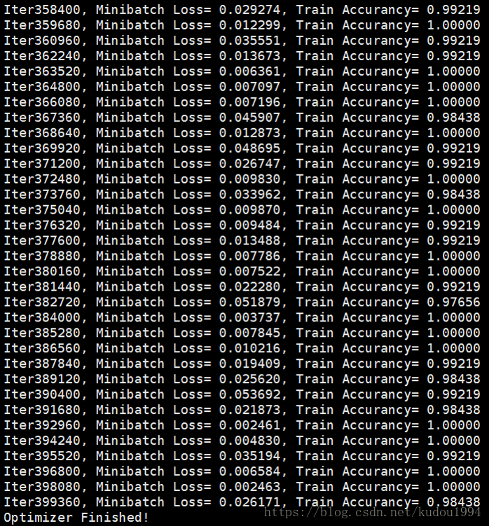

经过对比发现,在简单的图像识别方面,双向LSTM预测效果会更好。