一、算法简述
网络结构设计
通过创建MnistNet类,定义了包含两个卷积层和两个全连接层的深度神经网络。这个网络的设计灵感来自于经典的CNN结构,其中卷积层用于提取图像特征,而全连接层则用于将这些特征映射到最终的类别。
卷积与池化
卷积操作通过在输入图像上滑动卷积核,有效地捕捉图像的局部特征,例如边缘、纹理等。这种局部感知能力使得网络能够更好地理解输入图像的结构信息,从而更好地进行字符识别。在卷积操作后,激活函数的引入是为了引入非线性特性。ReLU激活函数通过将负值映射为零,保留正值,引入了非线性变换。这种非线性变换对于学习更加复杂的特征表示至关重要。池化层则在特征图上进行降维操作,最常见的是最大池化。最大池化通过在每个池化窗口中选择最大值,减小了特征图的尺寸,有助于提高模型的计算效率。此外,最大池化也有助于保留图像中最显著的特征,使网络对于空间变化更加鲁棒。
全连接层与激活函数
全连接层负责整合卷积层提取的特征,通过ReLU激活函数引入非线性。最终的全连接层输出通过Log_Softmax函数处理,转换为类别的概率分布。
Log_Softmax其实就是对Softmax取对数,表达式如下所示:

尽管,数学上log_Softmax是对Softmax取对数,但是,实际操作中是通过下面的式子来实现的:

其中,在加快运算速度的同时,保证数据的稳定性。
前向传播
在前向传播中,定义了输入数据如何在网络中传播。这个方法描述了数据如何通过卷积层、池化层和全连接层,最后经过Log Softmax函数的处理,网络的输出被转换为概率分布。Log Softmax对神经网络的输出进行归一化,使得每个类别的预测概率都落在 (0, 1) 的范围内,同时通过取对数的方式方便计算和优化。这一步为多类别分类问题提供了一种有效的建模方式。
网络参数
通过named_parameters方法,可以打印网络中所有参数的名称、值和大小,深入了解网络结构和模型的可训练参数,这样能够详细了解神经网络的结构。这对于验证网络是否按照预期的方式组织和连接层次非常有用。这种审查有助于确保网络的设计符合预期,并且每一层都按照计划进行连接。
MnistNet(
(conv1): Conv2d(1, 10, kernel_size=(5, 5), stride=(1, 1))
(conv2): Conv2d(10, 20, kernel_size=(3, 3), stride=(1, 1))
(fc1): Linear(in_features=2000, out_features=500, bias=True)
(fc2): Linear(in_features=500, out_features=10, bias=True)
)
二、设计步骤
本设计流程如下所示:

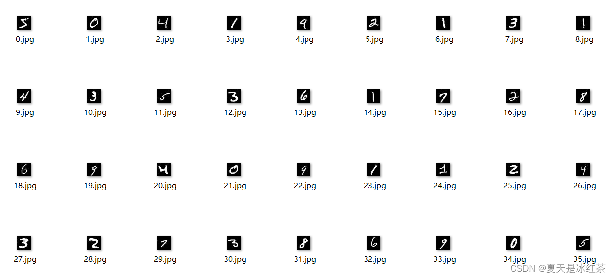
数据可视化及训练测试集划分
通过pytorch官方下载的MINIST数据集是以二进制的形式存放的,将数据集中的数字图像转换为jpg图像格式,可以更直观地展示和理解数据。更容易通过观察图像来理解和识别数字,而不是处理抽象的数字矩阵。在转化过程中,将图像路径和标签信息写入相应的文本文件中,以便后续的数据加载。
# Data_preprocessing.py

import torch
from torchvision import datasets, transforms
import os
from skimage import io
import torchvision.datasets.mnist as mnist

root = r"D:\PythonProject\pythonProject2\MNIST_pytorch\data\MNIST\raw"

#           下载测试集               #
train_dataset = datasets.MNIST('./data', train=True,
                               transform=transforms.Compose([
                                   transforms.ToTensor(),
                                   transforms.Normalize((0.1307,), (0.3081,))
                               ]),
                                download=True)

test_dataset = datasets.MNIST('./data', train=False,
                               transform=transforms.Compose([
                                   transforms.ToTensor(),
                                   transforms.Normalize((0.1307,), (0.3081,))
                               ]),
                                download=True)

train_set = (
    mnist.read_image_file(os.path.join(root, 'train-images-idx3-ubyte')),
    mnist.read_label_file(os.path.join(root, 'train-labels-idx1-ubyte'))
        )

test_set = (
    mnist.read_image_file(os.path.join(root, 't10k-images-idx3-ubyte')),
    mnist.read_label_file(os.path.join(root, 't10k-labels-idx1-ubyte'))
        )

def minist_to_img(train=True):
    if train:
        f = open(root+'train.txt','w')
        data_path=root+'/train/'
        if not os.path.exists(data_path):
            os.makedirs(data_path)
        for i, (img, label) in enumerate(zip(train_set[0], train_set[1])):
            img_path=data_path+str(i)+'.jpg'
            io.imsave(img_path, img.numpy())
            f.write(img_path+' ' + str(int(label)) + '\n')
        f.close()
    else:
        f = open(root + 'test.txt', 'w')
        data_path = root + '/test/'
        if not os.path.exists(data_path):
            os.makedirs(data_path)
        for i, (img,label) in enumerate(zip(test_set[0], test_set[1])):
            img_path = data_path + str(i) + '.jpg'
            io.imsave(img_path, img.numpy())
            f.write(img_path + ' ' + str(int(label)) + '\n')
        f.close()

#           数据划分                #
minist_to_img(True)    #  训练集
minist_to_img(False)   #  测试集
自定义数据加载器
# utils.py

import torch
from torchvision import transforms
from torch.utils.data import Dataset, DataLoader
from PIL import Image

class MINISTDataset(Dataset):
    def __init__(self, txtpath, transform=None):
        txt = open(txtpath, 'r')
        self.images = []
        for line in txt:
            line = line.strip('\n').rstrip().split()
            self.images.append((line[0], int(line[1])))
        self.transform = transform

    def __len__(self):
        return len(self.images)

    def __getitem__(self, idx):
        imgpath, label = self.images[idx]
        img = Image.open(imgpath).convert('L')
        if self.transform is not None:
            img = self.transform(img)
        return img, torch.tensor(label)


def MINISTDataloader(train_txtpath, test_txtpath, transform=None, batch_size=512):
    train_data = MINISTDataset(train_txtpath, transform)
    test_data = MINISTDataset(test_txtpath, transform)
    train_loader = DataLoader(dataset=train_data, batch_size=batch_size, shuffle=True)
    test_loader = DataLoader(dataset=test_data, batch_size=batch_size)
    return train_loader, test_loader


if __name__=="__main__":

    train_txtpath = r"D:\PythonProject\pythonProject2\MNIST_pytorch\data\MNIST\rawtrain.txt"
    test_txtpath = r"D:\PythonProject\pythonProject2\MNIST_pytorch\data\MNIST\rawtest.txt"
    transform=transforms.Compose([transforms.ToTensor(),
                                  transforms.Normalize((0.1307,), (0.3081,))
                                   ])
    train_loader, test_loader = MINISTDataloader(train_txtpath, test_txtpath, transform=transform, batch_size=512)
    print(len(train_loader))
    img, label = train_loader
    print(img, label)
通过包含图像文件路径和标签信息的文本文件路径来自定义数据加载器。在这里数据集格式每行包含一个图像文件路径和对应的标签信息,两者之间使用空格或其他分隔符分隔。例如,一行可以是:path/to/image1.jpg 0
其中 path/to/image1.jpg 是图像文件的路径,0是该图像的标签。通过索引加载将图像进行灰度,张量,归一化处理,对标签进行张量处理。最后,通过迭代数据加载器,可以获取包含图像和标签的批次数据,用于模型的训练和评估。
自定义MINIST网络
# net.py

import torch.nn as nn
import torch.nn.functional as F

class MnistNet(nn.Module):
    def __init__(self):
        super(MnistNet, self).__init__()
        self.conv1 = nn.Conv2d(1, 10, 5)
        self.conv2 = nn.Conv2d(10, 20, 3)
        self.fc1 = nn.Linear(20 * 10 * 10, 500)
        self.fc2 = nn.Linear(500, 10)  # 10分类

    def forward(self, x):
        in_size = x.size(0)           # BATCH_SIZE=512,输入的x:512*1*28*28。
        out = self.conv1(x)           # batch*1*28*28 -> batch*10*24*24(28x28的图像经过一次核为5x5的卷积,输出变为24x24)
        out = F.relu(out)             # batch*10*24*24
        out = F.max_pool2d(out, 2, 2)  # batch*10*24*24 -> batch*10*12*12(2*2的池化层会减半)
        out = self.conv2(out)         # batch*10*12*12 -> batch*20*10*10(再卷积一次,核的大小是3)
        out = F.relu(out)             # batch*20*10*10
        out = out.view(in_size, -1)   # batch*20*10*10 -> batch*2000(out的第二维是-1,进行自动推算)
        out = self.fc1(out)           # batch*2000 -> batch*500通过
        out = F.relu(out)             # batch*500
        out = self.fc2(out)           # batch*500 -> batch*10
        out = F.log_softmax(out, dim=1)  # 计算log(softmax(x))
        return out

if __name__=="__main__":
    net = MnistNet()
    print(net)
    for name, parameter in net.named_parameters():
        print(name, parameter, parameter.size())
在网络层结构,创建了两个卷积层conv1与conv2 ,一个输入通道数为1,输出通道数为10,卷积核大小为5x5。另一个输入通道数为10,输出通道数为20,卷积核大小为3x3。以及两个全连接层,一个输入大小为 20x10x10,输出大小为 500。另一个输入大小为 500,输出大小为 10。这里已知图像大小为28*28,批量假设为512,再经过一次核为5*5的卷积,输出变为24*24,通道数变为10,经过2*2最大池化层图像大小减半变为12*12,再卷积一次,核的大小为3,图像大小变为10*10,通道数变为20,然后经过relu非线性变化,但通道和尺寸均不变。最后将其平铺输入全连接层,起间经过一次relu非线性转换,通过Log_softmax计算概率。
神经网络训练与测试脚本解析
定义MinstNet,优化算法,损失函数,检查设备是否有cuda,使用自定义的数据加载器,对数据进行转换,将其转换为张量并进行像素值归一化。
# run.py

import torch
import torch.optim as optim
import torch.nn.functional as F

from MNIST_pytorch.utils import MINISTDataloader
from MNIST_pytorch.net import MnistNet
from torchvision import transforms

batch_size = 512
epochs = 20
device = torch.device("cuda" if torch.cuda.is_available() else "cpu")
net = MnistNet()
net = net.to(device)
optimizer = optim.Adam(net.parameters())
train_txtpath = r"D:\PythonProject\pythonProject2\MNIST_pytorch\data\MNIST\rawtrain.txt"
test_txtpath = r"D:\PythonProject\pythonProject2\MNIST_pytorch\data\MNIST\rawtest.txt"
transform=transforms.Compose([transforms.ToTensor(),
                              transforms.Normalize((0.1307,), (0.3081,))
                               ])

def train(model, device, train_loader, optimizer, epoch):
    model.train()
    for batch_idx, (data, target) in enumerate(train_loader):
        data, target = data.to(device), target.to(device)
        optimizer.zero_grad()
        output = model(data)
        loss = F.nll_loss(output, target)
        loss.backward()
        optimizer.step()
        if(batch_idx+1)%30 == 0:
            print('当前Train Epoch: {} [{}/{} ({:.0f}%)]\tLoss: {:.6f}'.format(
                epoch, batch_idx * len(data), len(train_loader.dataset),
                100. * batch_idx / len(train_loader), loss.item()))

def test(model, device, test_loader):
    model.eval()
    test_loss = 0
    correct = 0
    with torch.no_grad():
        for data, target in test_loader:
            data, target = data.to(device), target.to(device)
            output = model(data)
            test_loss += F.nll_loss(output, target, reduction='sum').item()
            pred = output.max(1, keepdim=True)[1] # 找到概率最大的下标
            correct += pred.eq(target.view_as(pred)).sum().item()

    test_loss /= len(test_loader.dataset)
    acc = correct / len(test_loader.dataset) * 100.
    print('\n验证集: Average loss: {:.4f}, Accuracy: {}/{} ({:.0f}%)\n'.format(
        test_loss, correct,
        len(test_loader.dataset), acc))

if __name__=="__main__":
    train_loader, test_loader = MINISTDataloader(train_txtpath, test_txtpath, transform, batch_size)
    for epoch in range(1, epochs + 1):
        train(net, device, train_loader, optimizer, epoch)
        test(net, device, test_loader)

        model_save_path = r"logs/model_weights.pth"
        torch.save(net.state_dict(), model_save_path)
        print(f'Model weights saved to {model_save_path}')

训练阶段,迭代训练数据集的批次。对于每个批次,执行以下操作:
- 将输入数据和目标标签移动到指定的设备。
- 将模型参数的梯度归零。
- 通过模型传递输入数据以获得预测。
- 计算预测和实际标签之间的负对数似然损失。
- 反向传播梯度并使用优化器更新模型参数。
- 每30个批次打印一次训练进度。
# val.py

import matplotlib.pyplot as plt
import numpy as np
import torch
import torch.nn.functional as F
import os
from MNIST_pytorch.utils import MINISTDataloader
from MNIST_pytorch.net import MnistNet
from torchvision import transforms
from matplotlib.font_manager import FontProperties

font_path = "msyh.ttc"
font_prop = FontProperties(fname=font_path)


batch_size = 512
device = torch.device("cuda" if torch.cuda.is_available() else "cpu")
net = MnistNet()
net = net.to(device)
train_txtpath = r"D:\PythonProject\pythonProject2\MNIST_pytorch\data\MNIST\rawtrain.txt"
test_txtpath = r"D:\PythonProject\pythonProject2\MNIST_pytorch\data\MNIST\rawtest.txt"
transform = transforms.Compose([transforms.ToTensor(),
                                transforms.Normalize((0.1307,), (0.3081,))
                                ])

def test(model, device, test_loader):
    model.eval()
    test_loss = 0
    correct = 0
    predictions = []
    ground_truth = []

    with torch.no_grad():
        for data, target in test_loader:
            data, target = data.to(device), target.to(device)
            output = model(data)
            test_loss += F.nll_loss(output, target, reduction='sum').item()
            pred = output.max(1, keepdim=True)[1]
            correct += pred.eq(target.view_as(pred)).sum().item()

            # 存储预测值和真实值,用于可视化
            predictions.extend(pred.cpu().numpy())
            ground_truth.extend(target.cpu().numpy())

    test_loss /= len(test_loader.dataset)
    acc = correct / len(test_loader.dataset) * 100.
    print('\n验证集: 平均损失: {:.4f}, 准确率: {}/{} ({:.0f}%)\n'.format(
        test_loss, correct,
        len(test_loader.dataset), acc))

    # 可视化来自验证集的一些随机样本
    num_samples = 5
    sample_indices = np.random.choice(len(test_loader.dataset), num_samples, replace=False)

    plt.figure(figsize=(12, 5))

    for i, idx in enumerate(sample_indices):
        data, target = test_loader.dataset[idx]
        data = data.to(device).unsqueeze(0)  # 添加额外的维度,因为模型期望一个批次
        output = model(data)
        predicted_label = output.argmax(dim=1).item()

        plt.subplot(1, num_samples, i + 1)
        plt.imshow(data.cpu().numpy().squeeze(), cmap='gray')
        plt.title(f'预测: {predicted_label}\n实际: {target.item()}',fontproperties=font_prop)
        plt.axis('off')

    plt.show()

    from sklearn.metrics import confusion_matrix
    import seaborn as sns

    cm = confusion_matrix(ground_truth, predictions)
    plt.figure(figsize=(10, 8))
    sns.heatmap(cm, annot=True, fmt='d', cmap='Blues', xticklabels=range(10), yticklabels=range(10))
    plt.xlabel('预测', fontproperties=font_prop)
    plt.ylabel('实际', fontproperties=font_prop)
    plt.title('混淆矩阵', fontproperties=font_prop)
    plt.show()

if __name__ == "__main__":
    model_weights_path = "logs/model_weights.pth"
    if os.path.exists(model_weights_path):
        net.load_state_dict(torch.load(model_weights_path))
        print(f'Model weights loaded from {model_weights_path}')
    else:
        print(f'No model weights found at {model_weights_path}. Please make sure to save the weights before testing.')
    train_loader, test_loader = MINISTDataloader(train_txtpath, test_txtpath, transform, batch_size)
    test(net, device, test_loader)
- 测试阶段,在测试数据集上评估训练好的模型。计算平均损失和准确性。期间,将模型设置为评估
- 模式(model.eval())来禁用dropout层和批量归一化。最后保存模型权重到指定的文件夹当中。
三、结果分析
训练集样本数量为6万,测试集样本数量为1万,批次为512,训练轮次为20,对数据进行张量,归一化处理。
训练和测试结果如下所示:

图 1 训练及测试阶段损失变化
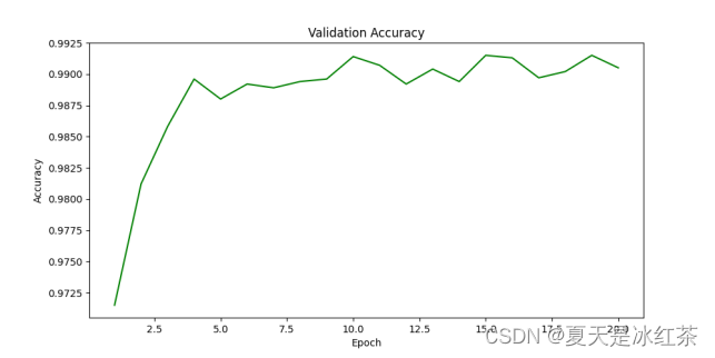
图 2 验证集正确率
# plot.py


import matplotlib.pyplot as plt

train_losses = [0.260449, 0.077057, 0.083472, 0.044373, 0.031067, 0.035871,
                0.009805, 0.010832, 0.006299, 0.006840, 0.001358, 0.003195,
                0.005098, 0.002992, 0.002009, 0.000739, 0.006418, 0.002669,
                0.000109, 0.000568]  # 填入训练过程中的损失值列表
valid_losses = [0.0920, 0.0563, 0.0440, 0.0339, 0.0362, 0.0352, 0.0341, 0.0335,
                0.0347, 0.0301, 0.0330, 0.0370, 0.0354, 0.0365, 0.0298, 0.0328,
                0.0388, 0.0410, 0.0337, 0.0382]  # 填入验证集的损失值列表
valid_accuracies = [9715/10000, 9812/10000, 9858/10000, 9896/10000, 9880/10000,
                    9892/10000, 9889/10000, 9894/10000, 9896/10000, 9914/10000,
                    9907/10000, 9892/10000, 9904/10000, 9894/10000, 9915/10000,
                    9913/10000, 9897/10000, 9902/10000, 9915/10000, 9905/10000]  # 填入验证集的准确率列表

epochs = range(1, len(train_losses) + 1)

# 损失值曲线
plt.figure(figsize=(10, 5))
plt.plot(epochs, train_losses, 'b', label='Training Loss')
plt.plot(epochs, valid_losses, 'r', label='Validation Loss')
plt.title('Training and Validation Loss')
plt.xlabel('Epoch')
plt.ylabel('Loss')
plt.legend()
plt.show()

# 准确率曲线
plt.figure(figsize=(10, 5))
plt.plot(epochs, valid_accuracies, 'g')
plt.title('Validation Accuracy')
plt.xlabel('Epoch')
plt.ylabel('Accuracy')
plt.show()
这里的train_loss,vaild_loss,vaild_accuracies均来自于训练过程。
由图1图2可知,损失下降很快,正确率很快就上升了,这可能与数据集比较简单有关。

图 3 加载模型权重验证
这里随机选择了五张图片进行测试,五张均正确分类,说明我设计的模型在这个小样本上表现很好。

图 4 混淆矩阵
由图4混淆矩阵对角线上的值都比其他地方大时,说明我的模型在训练数据集上表现良好,能够正确地预测大多数样本的类别。对角线上的元素表示模型在相应类别上的正确分类数量。高的 TP 值表示模型成功地识别了这些类别的样本。
四、结论
本次设计了一个深度神经网络,包括两个卷积层和两个全连接层,以及适当的激活函数和池化层。该结构能够有效地提取手写字符图像的特征,并通过Log Softmax函数将输出转换为概率分布。在训练集上,模型在20个轮次内取得了显著的损失下降,并在验证集上达到了高准确率。测试集结果表明,模型在未见过的数据上也能够良好地泛化,对手写字符进行准确的识别。通过加载保存的模型权重进行验证,我们成功地对随机选择的五张手写字符图像进行了测试,所有测试样本均被正确分类。这表明我们的模型在实际应用中表现良好。在分析混淆矩阵时,发现对角线上的值比其他地方大,说明模型在训练数据集上表现良好,能够正确地预测大多数样本的类别。
手写字符识别模型在设计和实现中取得了令人满意的成果,展现了深度学习和神经网络技术在图像识别领域的应用潜力。
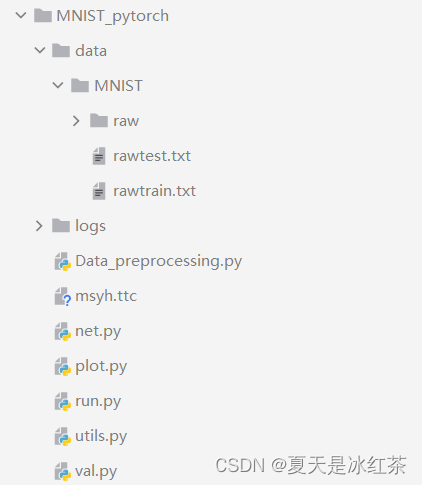
五、项目目录结构