【强化学习】18 —— SAC（ Soft Actor-Critic）

前言

之前的章节提到过在线策略算法的采样效率比较低，我们通常更倾向于使用离线策略算法。然而，虽然 DDPG 是离线策略算法，但是它的训练非常不稳定，收敛性较差，对超参数比较敏感，也难以适应不同的复杂环境。2018 年，一个更加稳定的离线策略算法 Soft Actor-Critic（SAC）被提出。SAC 的前身是 Soft Q-learning，它们都属于最大熵强化学习的范畴。Soft Q-learning 不存在一个显式的策略函数，而是使用一个函数$Q$的波尔兹曼分布，在连续空间下求解非常麻烦。于是 SAC 提出使用一个 Actor 表示策略函数，从而解决这个问题。目前，在无模型的强化学习算法中，SAC 是一个非常高效的算法，它学习一个随机性策略，在不少标准环境中取得了领先的成绩。

最大熵强化学习

熵是策略中随机性的一种度量，设$x$为随机变量，概率密度函数为$P$，熵$H$的计算式为：$$H(p)={\mathbb{E}}_{x\sim p}[-\log p(x)]$$在强化学习中，我们可以使用$H(\pi (\cdot |s))$来表示策略$\pi$在状态$s$下的随机程度。最大熵强化学习（maximum entropy RL）的思想就是除了要最大化累积奖励，还要使得策略更加随机，除此之外还要增加算法的鲁棒性以及提升策略的预训练效果。

传统的RL难以适应于复杂变化的环境。如图所示，通过学习，智能体会倾向于选择上面的路径（因为更短），但若在上方的通道设置一个障碍，智能体则无法通过，且需重新学习下方的路径以达到终点。

如图3a所示，传统的RL策略类似于一个单峰的高斯分布，而最大熵强化学习则是类似于3b中所示的多峰分布。前者会忽视掉其他较低概率的策略，而后者则是增加了对其他的策略的探索，使之能够适应更复杂的环境。

不同动作空间下的最大熵强化学习

离散动作空间
在最大熵强化学习中，带有最大熵的目标函数通过增加一个熵项，使得最优策略的熵在每次迭代下达到最大。
$$\begin{array}{rl}{\pi }_{\mathrm{MaxEnt}}^{\ast }=& \arg \underset{\pi }{\max }\sum _t{\mathbb{E}}_{({\mathbf{s}}_t,{\mathbf{a}}_t)\sim {\rho }_{\pi }}\left[r({\mathbf{s}}_t,{\mathbf{a}}_t)+\alpha \mathcal{H}(\pi (\cdot |{\mathbf{s}}_t))\right]\end{array}$$$$\mathcal{H}(\pi (\cdot |s_t))=-\sum _{a_t}\pi (a_t|s_t)\log (\pi (a_t|s_t))$$其中，$\alpha$是一个正则化的系数，用来控制熵的重要程度。熵正则化增加了强化学习算法的探索程度，当$\alpha =0$时，最大熵强化学习与传统的 RL算法相同;当$\alpha >0$时，$\alpha$越大，探索性就越强，有助于加速后续的策略学习，并减少策略陷入较差的局部最优的可能性，鲁棒性越好。

⚠️You Should Know
请注意，优化目标与玻尔兹曼探索(Sallans & Hinton, 2004)和PGQ (O’Donoghue et al.， 2016)的行为有质的不同，后者基于贪婪策略在当前时间步长最大化熵，但没有明确会优化未来可能到达高熵状态的策略。这个不同之处很重要，因为最大熵优化目标会最大化策略$\pi$的整个轨迹的熵。

连续动作空间
$$a=\mu (\cdot |s_t)+ϵ$$
对于连续动作空间，通常会加上噪声项$ϵ$，以增强算法的探索能力。$ϵ$通常是一个高斯分布。但是这种方法会有难以学到多样化的策略$\mu$以及因为$ϵ$服从预定义的分布，而难以泛化到多模态的复杂情况等问题。

基于能量的模型

优化最大熵目标为我们提供了一个训练随机策略的框架，但是其中的策略还未进行表示。以往的工作中有采用多项分布或者高斯分布进行表示，然而，如果我们想使用一类通用的分布来表示复杂的、多模态的行为，我们可以选择使用这种形式的基于能量的通用策略：$$\pi ({\mathbf{a}}_t|{\mathbf{s}}_t)\propto \exp \left(-\mathcal{E}({\mathbf{s}}_t,{\mathbf{a}}_t)\right),$$

其中，$\mathcal{E}$代表能量函数，可用深度神经网络进行拟合。接下来简要介绍一下基于能量的模型。

基于能量的模型(Energy-Based Model, EBM)的目标是最大化打分函数$\varphi (x)$的期望，同时增加探索性：
$$\underset{p}{\max }{\mathbb{E}}_{x\sim p}[\varphi (x)]+\alpha \mathcal{H}(p)$$

其中，$\alpha$越大，越鼓励探索。最终求解出的分布符合波兹曼分布(Boltzmann distribution)$，p^{\ast }(x)\propto e^{-\varphi (x)/\alpha }$（其中$\alpha$又可以被称为温度系数）。将目标函数除以$\alpha$，因为$H(p)={\mathbb{E}}_{x\sim p}[-\log p(x)]$，将两项合并，最终最大化目标函数等价于最小化负的$p$和$p_{\varphi }$的KL散度。
$$\frac{{\mathbb{E}}_{x\sim p}[\varphi (x)]}{\alpha }+\mathcal{H}(p)={\mathbb{E}}_{x\sim p}\left[\frac{\varphi (x)}{\alpha }-\log p(x)\right]=-KL(p||p_{\varphi })$$

波兹曼分布(Boltzmann distribution)$p_{\varphi }(x)=\frac{e^{\varphi (x)/\alpha }}{z}=\frac{e^{-\epsilon (x)}}{z}$的能量函数为$\epsilon (x)=-\frac{\varphi (x)}{\alpha }$，能量越高越不确定。

在最大熵强化学习中，策略优化目标为（即，令$\mathcal{E}(s_t,a_t)=-\frac{1}{\alpha }{Q}_{soft}(s_t,a_t)$）：
$$\underset{a}{\max }{\mathbb{E}}_{x\sim \pi (\cdot |s)}[Q(s,a)]+\alpha \mathcal{H}(\pi (\cdot |s))$$因此，最大熵强化学习不会像传统RL那样直接选取最大的Q函数值，而是将探索性考虑进来，从而避免陷入局部最小值。在实践应用中,最大熵的优点包括:1)它鼓励更广泛的探索,同时放弃多余的样本;2)该策略可以得到多个近似最优动作;3)该方法可以有效地提高训练速度,是优化传统RL目标函数的一种新方法。

软价值函数

考虑到熵的因素，我们可以对价值函数做一些变更：
$$V^{\pi }(s)=E_{\tau \sim \pi }\sum _{t=0}^{\infty }{\gamma }^t(R(s_t,a_t,s_{t+1})+\alpha H\left(\pi (\cdot |s_t)\right))|s_0=s$$$$Q^{\pi }(s,a)=E_{\tau \sim \pi }\sum _{t=0}^{\infty }{\gamma }^{t}R(s_t,a_t,s_{t+1})+\alpha \sum _{t=1}^{\infty }{\gamma }^{t}H\left(\pi (\cdot |s_t)\right)|s_0=s,a_0=a$$

相应的bellman方程为：
$$V^{\pi }(s)=E_{a\sim \pi }{Q}^{\pi }(s,a)+\alpha H\left(\pi (\cdot |s)\right)$$$$\begin{array}{rl}{Q}^{\pi }(s,a)=& E_{s^{\prime }\sim P,a^{\prime }\sim \pi }[R(s,a,s^{\prime })+\gamma \left(Q^{\pi }(s^{\prime },a^{\prime })+\alpha H\left(\pi (\cdot |s^{\prime })\right)\right)]\\ =& E_{s^{\prime }\sim P}[R(s,a,s^{\prime })+\gamma V^{\pi }(s^{\prime })].\end{array}$$

最大熵策略

最大熵强化学习的策略目标是${\max }_a{\mathbb{E}}_{x\sim \pi (\cdot |s)}[Q_{soft}(s,a)]+\alpha \mathcal{H}(\pi (\cdot |s))$，基于能量模型的形式 ，则可表示为
$${\pi }_{\mathrm{Maxlnt}}(a|s)\propto \exp (Q_{soft}(s,a)/\alpha )$$
状态值函数的具体形式为：
$$\begin{array}{rl}{V}_{soft}(s_t)& ={\mathbb{E}}_{a\sim \pi }[Q_{soft}(s_t,a_t)]+\alpha \mathcal{H}(\pi (\cdot |s_t))\\ V_{soft}(s_t)& \leftarrow \alpha \log \int \exp \left(\frac{1}{\alpha }{Q}_{soft}(s_t,a^{\prime })\right)d{a}^{\prime }\end{array}$$

基于此的最优策略为：

$${\pi }_{\mathrm{Maxlnt}}(a|s)=\exp \left(\frac{1}{\alpha }(Q_{soft}^{\ast }(s_t,a_t)-V_{soft}^{\ast }(s_t))\right)$$

⚠️You Should Know
证明过程可参考 Reinforcement Learning with Deep Energy-Based Policies, 2017, arXiv

Soft Q-learning

Soft Q-Iteration

类似于Q-learning，通过对$Q_{soft}^{}$以及$V_{soft}^{}$的不断迭代，可以使得结果不断向收敛至$Q_{soft}^{\ast }$和$V_{soft}^{\ast }$以及$\pi \to {\pi }_{\mathrm{MaxEnt}}^{\ast }$。$$\begin{array}{r}{Q}_{\mathrm{soft}}({\mathbf{s}}_t,{\mathbf{a}}_t)\leftarrow r_t+\gamma {\mathbb{E}}_{{\mathbf{s}}_{t+1}\sim p_{\mathbf{s}}}\left[V_{\mathrm{soft}}({\mathbf{s}}_{t+1})\right],\forall {\mathbf{s}}_t,{\mathbf{a}}_t(8)\\ V_{\mathrm{soft}}({\mathbf{s}}_t)\leftarrow \alpha \log {\int }_{\mathcal{A}}\exp \left(\frac{1}{\alpha }{Q}_{\mathrm{soft}}({\mathbf{s}}_t,{\mathbf{a}}^{\prime })\right)d{\mathbf{a}}^{\prime },\forall {\mathbf{s}}_t(9)\end{array}$$$convergesto{Q}_{\mathrm{soft}}^{\ast }and{V}_{\mathrm{soft}}^{\ast },respectively.$

⚠️You Should Know
收敛性证明过程可参考 Reinforcement Learning with Deep Energy-Based Policies, 2017, arXiv

但是上述软贝尔曼更新（soft Bellman backup）的方式不能精确地在连续或大的状态和动作空间中执行，其次基于能量模型进行采样是比较困难的。

Soft Q-Learning

由于(9)中存在的积分以及存在无限的状态和动作集合，上述过程难以实现，因此，作者使用了随机优化的方法进行描述，同时上述过程变为了一个随机梯度下降更新过程。Soft Q-function可以被建模成关于参数$\theta$的函数$Q_{soft}^{\theta }(s_t,a_t)$。为了描述上述的随机过程，Soft Q-Learning使用了重要性采样对价值函数进行描述：$$V_{\text{soft}}^{\theta }({\mathbf{s}}_t)=\alpha \log {\mathbb{E}}_{\pi }\left[\frac{\exp \left(\frac{1}{\alpha }{Q}_{\text{soft}}^{\theta }({\mathbf{s}}_t,{\mathbf{a}}^{\prime })\right)}{\pi ({\mathbf{a}}^{\prime })}\right]$$

$\pi$可以表示为任意的策略分布。之后利用均方误差计算目标函数，${\hat{Q}}_{\mathrm{soft}}^{\bar{\theta }}({\mathbf{s}}_t,{\mathbf{a}}_t)=r_t+\gamma {\mathbb{E}}_{{\mathbf{s}}_{t+1}\sim p_{\mathbf{s}}}[V_{\mathrm{soft}}^{\bar{\theta }}({\mathbf{s}}_{t+1})]$为目标的Q-值：

$$J_Q(\theta )={\mathbb{E}}_{{\mathbf{s}}_t\sim q_{{\mathbf{s}}_t},{\mathbf{a}}_t\sim q_{{\mathbf{a}}_t}}\left[\frac{1}{2}{\left({\hat{Q}}_{\mathrm{soft}}^{\bar{\theta }}({\mathbf{s}}_t,{\mathbf{a}}_t)-Q_{\mathrm{soft}}^{\theta }({\mathbf{s}}_t,{\mathbf{a}}_t)\right)}^2\right]$$

⚠️You Should Know
因为$q_{{\mathbf{s}}_t},q_{{\mathbf{a}}_t}$采样的分布可以是任意的。通常来说可以基于当前policy的一些rollouts进行采样$\pi ({\mathbf{a}}_t|{\mathbf{s}}_t)\propto \exp \left(\frac{1}{\alpha }{Q}_{\mathrm{soft}}^{\theta }({\mathbf{s}}_t,{\mathbf{a}}_t)\right)$。
对于$\pi$的分布，通常来说可以采用均匀分布，但更好的选择是使用当前策略，以达到无偏估计的效果。

近似采样与SVGD

然而，在连续空间中，我们仍然需要一种可行的方法来从策略$\pi ({\mathbf{a}}_t|{\mathbf{s}}_t)\propto \exp \left(\frac{1}{\alpha }{Q}_{\mathrm{soft}}^{\theta }({\mathbf{s}}_t,{\mathbf{a}}_t)\right)$中采样，不仅用于采取策略$\pi$的行为，还可以在需要时生成动作样本以估计软值函数。由于策略的形式非常广泛，因此直接从它中采样是不可行的。因此需要一种近似采样的方法。

以往的方案大致可以分为两类：基于马尔可夫链蒙特卡罗(MCMC)的采样；从目标分布中训练输出近似样本的随机抽样网络。但是MCMC的方法不太适用于在线推理过程，因此作者将使用Stein variational gradient descent (SVGD) 和amortized SVGD的采样网络。Amortized SVGD有一些比较有趣的性质：

1. 它为我们提供了一个随机体素网络，可以用于极快地生成样本。
2. 它可以证明会收敛到 EBM 的后验分布的准确估计
3. 该算法类似于actor-critic算法

通过学习一个状态条件随机神经网络 $a_t=f^{\varphi }(\xi ;s_t)$，由 $\varphi$ 参数化，它将从正常高斯或其他任意分布中提取的噪声样本 $\xi$ 映射到对应于 $Q_{soft}^{\theta }$ 的目标 EBM 的无偏动作样本。将学习到的策略标为${\pi }^{\varphi }(s_t,a_t)$，通过KL 散度（KL divergence）进行近似：$$\begin{array}{rl}{J}_{\pi }(\varphi ;s_t)& =KL\left({\pi }^{\varphi }(\cdot |s_t)||\exp \left(\frac{1}{\alpha }(Q_{soft}^{\theta }(s_t,\cdot )-V_{soft}^{\theta })\right)\right)\\ a_t& =f^{\varphi }(\xi ;s_t),\xi \sim \mathcal{N}\end{array}$$

SVGD的方法提供了贪婪的搜索策略：$$\begin{array}{c}\Delta f^{\varphi }(\cdot ;{\mathbf{s}}_t)={\mathbb{E}}_{{\mathbf{a}}_t\sim {\pi }^{\varphi }}{\left|\kappa ({\mathbf{a}}_t,f^{\varphi }(\cdot ;{\mathbf{s}}_t)){\nabla }_{{\mathbf{a}}^{\prime }}{Q}_{\mathrm{soft}}^{\theta }({\mathbf{s}}_t,{\mathbf{a}}^{\prime })\right|}_{{\mathbf{a}}^{\prime }={\mathbf{a}}_t}\\ +\alpha {{\nabla }_{{\mathbf{a}}^{\prime }}\kappa ({\mathbf{a}}^{\prime },f^{\varphi }(\cdot ;{\mathbf{s}}_t))|}_{{\mathbf{a}}^{\prime }={\mathbf{a}}_t}],\end{array}$$

之后使用链式法则，并将SVGD反向传播到策略网络中，并使用任意基于梯度的优化方法来学习最优采样网络参数。$$\frac{\partial J_{\pi }(\varphi ;{\mathbf{s}}_t)}{\partial \varphi }\propto {\mathbb{E}}_{\xi }\left[\Delta f^{\varphi }(\xi ;{\mathbf{s}}_t)\frac{\partial f^{\varphi }(\xi ;{\mathbf{s}}_t)}{\partial \varphi }\right],$$

⚠️You Should Know
$\Delta f^{\varphi }$不是严格的策略梯度，而是核函数$\kappa$再现核希尔伯特空间（reproducing kernel Hilbert space）的最优方向

伪代码

Soft Actor-Critic

Haarnoja T, Zhou A, Abbeel P, et al. Soft actor-critic: Off-policy maximum entropy deep reinforcement learning with a stochastic actor[C]//International conference on machine learning. PMLR, 2018: 1861-1870.

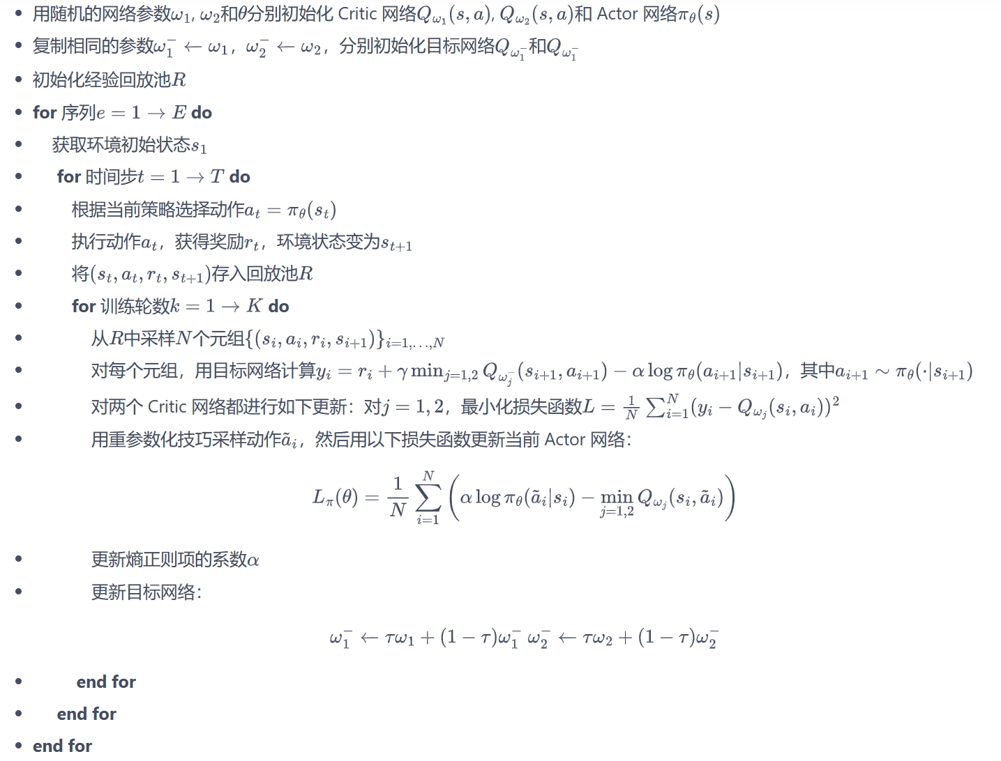
用SVGD做近似推断可能存在需要对随机数的分布进行假设的问题同时会使得复杂度和不稳定性提升。除此之外，相比策略梯度或者actor-critic等算法，近似推断可能不那么直接与有效。SAC对策略和价值函数都进行了函数逼近，通过交替使用随机梯度下降优化两个网络。以下是相关算法细节：

价值函数学习目标：

$$\begin{array}{c}{J}_V(\psi )={\mathbb{E}}_{s_t\sim \mathcal{D}}\left[\frac{1}{2}(V_{\psi }(s_t)-{\mathbb{E}}_{a_t\sim {\pi }_{\varphi }}[Q_{\theta }(s_t,a_t)-\log {\pi }_{\varphi }(a_t|s_t)]{)}^2\right]\\ J_Q(\theta )={\mathbb{E}}_{(s_t,a_t)\sim \mathbb{D}}\left[\frac{1}{2}{\left(r(s_t,a_t)+\gamma {\mathbb{E}}_{s_{t+1}\sim p}[V_{\overline{\psi }}(s_{t+1})]-Q_{\theta }(s_t,a_t)\right)}^2\right]\end{array}$$

策略函数学习目标：$$\begin{array}{r}{J}_{\pi }(\varphi )={\mathbb{E}}_{{\mathbf{s}}_t\sim \mathcal{D},{ϵ}_t\sim \mathcal{N}}[\log {\pi }_{\varphi }(f_{\varphi }({ϵ}_t;{\mathbf{s}}_t)|{\mathbf{s}}_t)-Q_{\theta }({\mathbf{s}}_t,f_{\varphi }({ϵ}_t;{\mathbf{s}}_t))]\end{array}$$

利用两个动作价值函数网络，每次使用Q网络时，使用较小的那一个：$$\begin{array}{rl}{L}_Q(\omega )& ={\mathbb{E}}_{(s_t,a_t,r_t,s_{t+1})\sim R}\left[\frac{1}{2}{\left(Q_{\omega }(s_t,a_t)-(r_t+\gamma V_{{\omega }^{-}}(s_{t+1}))\right)}^2\right]\\ & ={\mathbb{E}}_{(s_t,a_t,r_t,s_{t+1})\sim R,a_{t+1}\sim {\pi }_{\theta }(\cdot |s_{t+1})}\left[\frac{1}{2}{\left(Q_{\omega }(s_t,a_t)-(r_t+\gamma (\underset{j=1,2}{\min }{Q}_{{\omega }_j^{-}}(s_{t+1},a_{t+1})-\alpha \log \pi (a_{t+1}|s_{t+1})))\right)}^2\right]\end{array}$$

重参数化技巧与自动调整熵正则项参考《动手学强化学习》SAC 算法

伪代码

代码实践

连续动作空间

import gymnasium as gym
import numpy as np
from tqdm import tqdm
import torch
import torch.nn.functional as F
import util

class PolicyNetContinuous(torch.nn.Module):
    def __init__(self, state_dim, hidden_dim, action_dim, action_bound):
        super(PolicyNetContinuous, self).__init__()
        self.fc1 = torch.nn.Linear(state_dim, hidden_dim)
        self.mu = torch.nn.Linear(hidden_dim, action_dim)
        self.std = torch.nn.Linear(hidden_dim, action_dim)
        self.action_bound = action_bound

    def forward(self, x):
        x = F.relu(self.fc1(x))
        mu = self.mu(x)
        std = F.softplus(self.std(x))
        dist = torch.distributions.Normal(mu, std)
        normal_sample = dist.rsample()  # rsample()是重参数化采样
        log_prob = dist.log_prob(normal_sample)
        action = torch.tanh(normal_sample)
        # 计算tanh_normal分布的对数概率密度
        log_prob = log_prob - torch.log(1 - torch.tanh(action).pow(2) + 1e-7)
        action = action * self.action_bound
        return action, log_prob

class QValueNetContinuous(torch.nn.Module):
    def __init__(self, state_dim, hidden_dim, action_dim):
        super(QValueNetContinuous, self).__init__()
        self.fc1 = torch.nn.Linear(state_dim + action_dim, hidden_dim)
        self.fc2 = torch.nn.Linear(hidden_dim, hidden_dim)
        self.fc_out = torch.nn.Linear(hidden_dim, 1)

    def forward(self, x, a):
        cat = torch.cat([x, a], dim=1)
        x = F.relu(self.fc1(cat))
        x = F.relu(self.fc2(x))
        return self.fc_out(x)

class SACContinuous:
    ''' 处理连续动作的SAC算法 '''
    def __init__(self, state_dim, hidden_dim, action_dim, action_bound, actor_lr, critic_lr, gamma,
                 alpha_lr, target_entropy, tau, buffer_size, minimal_size, batch_size,
                 device, numOfEpisodes, env):
        self.actor = PolicyNetContinuous(state_dim, hidden_dim, action_dim, action_bound).to(device)
        self.critic_1 = QValueNetContinuous(state_dim, hidden_dim, action_dim).to(device)
        self.critic_2 = QValueNetContinuous(state_dim, hidden_dim, action_dim).to(device)
        self.target_critic_1 = QValueNetContinuous(state_dim, hidden_dim, action_dim).to(device)
        self.target_critic_2 = QValueNetContinuous(state_dim, hidden_dim, action_dim).to(device)
        # 令目标Q网络的初始参数和Q网络一样
        self.target_critic_1.load_state_dict(self.critic_1.state_dict())
        self.target_critic_2.load_state_dict(self.critic_2.state_dict())
        self.actor_optimizer = torch.optim.Adam(self.actor.parameters(), lr=actor_lr)
        self.critic_1_optimizer = torch.optim.Adam(self.critic_1.parameters(), lr=critic_lr)
        self.critic_2_optimizer = torch.optim.Adam(self.critic_2.parameters(), lr=critic_lr)
        # 使用alpha的log值,可以使训练结果比较稳定
        self.log_alpha = torch.tensor(np.log(0.01), dtype=torch.float)
        self.log_alpha.requires_grad = True  # 可以对alpha求梯度
        self.log_alpha_optimizer = torch.optim.Adam([self.log_alpha], lr=alpha_lr)
        self.target_entropy = target_entropy
        self.gamma = gamma
        self.tau = tau
        self.device = device
        self.env = env
        self.numOfEpisodes = numOfEpisodes
        self.buffer_size = buffer_size
        self.minimal_size = minimal_size
        self.batch_size = batch_size

    def take_action(self, state):
        state = torch.FloatTensor(np.array([state])).to(self.device)
        action = self.actor(state)[0]
        return [action.item()]

    def calc_target(self, rewards, next_states, terminateds, truncateds):
        next_action, log_prob = self.actor(next_states)
        entropy = -log_prob
        q1_value = self.target_critic_1(next_states, next_action)
        q2_value = self.target_critic_2(next_states, next_action)
        next_value = torch.min(q1_value, q2_value) + self.log_alpha.exp() * entropy
        td_target = rewards + self.gamma * next_value * (1 - terminateds + truncateds)
        return td_target

    def soft_update(self, net, target_net):
        for param_target, param in zip(target_net.parameters(), net.parameters()):
            param_target.data.copy_(param_target.data * (1.0 - self.tau) + param.data * self.tau)

    def update(self, transition_dict):
        states = torch.tensor(np.array(transition_dict['states']), dtype=torch.float).to(self.device)
        actions = torch.tensor(np.array(transition_dict['actions']), dtype=torch.float).view(-1, 1).to(self.device)
        rewards = torch.tensor(transition_dict['rewards'], dtype=torch.float).view(-1, 1).to(self.device)
        next_states = torch.tensor(np.array(transition_dict['next_states']), dtype=torch.float).to(self.device)
        terminateds = torch.tensor(transition_dict['terminateds'], dtype=torch.float).view(-1, 1).to(self.device)
        truncateds = torch.tensor(transition_dict['truncateds'], dtype=torch.float).view(-1, 1).to(self.device)
        rewards = (rewards + 8.0) / 8.0
        # 更新两个Q网络
        td_target = self.calc_target(rewards, next_states, terminateds, truncateds)
        critic_loss1 = torch.mean(F.mse_loss(td_target.detach(), self.critic_1(states, actions)))
        critic_loss2 = torch.mean(F.mse_loss(td_target.detach(), self.critic_2(states, actions)))
        self.critic_1_optimizer.zero_grad()
        critic_loss1.backward()
        self.critic_1_optimizer.step()
        self.critic_2_optimizer.zero_grad()
        critic_loss2.backward()
        self.critic_2_optimizer.step()
        # 更新策略网络
        new_actions, log_prob = self.actor(states)
        entropy = -log_prob
        q1_value = self.critic_1(states, new_actions)
        q2_value = self.critic_2(states, new_actions)
        next_value = torch.min(q1_value, q2_value)
        actor_loss = torch.mean(-self.log_alpha.exp() * entropy - next_value)
        self.actor_optimizer.zero_grad()
        actor_loss.backward()
        self.actor_optimizer.step()
        # 更新alpha值
        alpha_loss = torch.mean(self.log_alpha.exp() * (entropy - self.target_entropy).detach())
        self.log_alpha_optimizer.zero_grad()
        alpha_loss.backward()
        self.log_alpha_optimizer.step()

        self.soft_update(self.critic_1, self.target_critic_1)
        self.soft_update(self.critic_2, self.target_critic_2)

    def SACtrain(self):
        replay_buffer = util.ReplayBuffer(self.buffer_size)
        returnList = []
        for i in range(10):
            with tqdm(total=int(self.numOfEpisodes / 10), desc='Iteration %d' % i) as pbar:
                for episode in range(int(self.numOfEpisodes / 10)):
                    # initialize state
                    state, info = self.env.reset()
                    terminated = False
                    truncated = False
                    episodeReward = 0
                    # Loop for each step of episode:
                    while (not terminated) or (not truncated):
                        action = self.take_action(state)
                        next_state, reward, terminated, truncated, info = self.env.step(action)
                        replay_buffer.add(state, action, reward, next_state, terminated, truncated)
                        state = next_state
                        episodeReward += reward
                        # 当buffer数据的数量超过一定值后,才进行Q网络训练
                        if replay_buffer.size() > self.minimal_size:
                            b_s, b_a, b_r, b_ns, b_te, b_tr = replay_buffer.sample(self.batch_size)
                            transition_dict = {
    
    
                                'states': b_s,
                                'actions': b_a,
                                'next_states': b_ns,
                                'rewards': b_r,
                                'terminateds': b_te,
                                'truncateds': b_tr
                            }
                            self.update(transition_dict)
                        if terminated or truncated:
                            break
                    returnList.append(episodeReward)
                    if (episode + 1) % 10 == 0:  # 每10条序列打印一下这10条序列的平均回报
                        pbar.set_postfix({
    
    
                            'episode':
                                '%d' % (self.numOfEpisodes / 10 * i + episode + 1),
                            'return':
                                '%.3f' % np.mean(returnList[-10:])
                        })
                    pbar.update(1)
        return returnList

def test01():
    device = torch.device("cuda") if torch.cuda.is_available() else torch.device("cpu")
    env = gym.make("Pendulum-v1")
    agent = SACContinuous(state_dim=env.observation_space.shape[0],
                          hidden_dim=256,
                          action_dim=env.action_space.shape[0],
                          action_bound=env.action_space.high[0],
                          actor_lr=3e-4,
                          critic_lr=3e-3,
                          gamma=0.99,
                          alpha_lr=3e-4,
                          target_entropy=-env.action_space.shape[0],
                          tau=0.005,
                          buffer_size=100000,
                          minimal_size=1000,
                          batch_size=64,
                          device=device,
                          numOfEpisodes=200,
                          env=env)
    returnLists1 = agent.SACtrain()
    ReturnList = []
    ReturnList.append(util.smooth([returnLists1], sm=20))
    labelList = ['SAC']
    util.PlotReward(200, ReturnList, labelList, 'Pendulum-v1')
    np.save("D:\LearningRL\Hands-on-RL\SAC_Pendulum\ReturnData\SAC_v1_1.npy", returnLists1)
    env.close()

结果：

可以看到SAC在连续动作空间的任务中表现优秀。

离散动作空间

⚠️You Should Know
对于离散的动作空间，策略网络和价值网络的网络结构将发生如下改变：

• 策略网络的输出修改为在离散动作空间上的 softmax 分布；
  该策略网络输出一个离散的动作分布，所以在价值网络的学习过程中，不需要再对下一个动作$a_{t+1}$进行采样，而是直接通过概率计算来得到下一个状态的价值。同理，在$\alpha$的损失函数计算中，也不需要再对动作进行采样。
• 价值网络直接接收状态和离散动作空间的分布作为输入。

class PolicyNet(torch.nn.Module):
    def __init__(self, state_dim, hidden_dim, action_dim):
        super(PolicyNet, self).__init__()
        self.fc1 = torch.nn.Linear(state_dim, hidden_dim)
        self.fc2 = torch.nn.Linear(hidden_dim, action_dim)

    def forward(self, x):
        x = F.relu(self.fc1(x))
        return F.softmax(self.fc2(x), dim=1)

class QValueNet(torch.nn.Module):
    ''' 只有一层隐藏层的Q网络 '''
    def __init__(self, state_dim, hidden_dim, action_dim):
        super(QValueNet, self).__init__()
        self.fc1 = torch.nn.Linear(state_dim, hidden_dim)
        self.fc2 = torch.nn.Linear(hidden_dim, action_dim)

    def forward(self, x):
        x = F.relu(self.fc1(x))
        return self.fc2(x)

class SACContinuous:
    ''' 处理连续动作的SAC算法 '''
    def __init__(self, state_dim, hidden_dim, action_dim, actor_lr, critic_lr, gamma,
                 alpha_lr, target_entropy, tau, buffer_size, minimal_size, batch_size,
                 device, numOfEpisodes, env):
        self.actor = PolicyNet(state_dim, hidden_dim, action_dim).to(device)
        self.critic_1 = QValueNet(state_dim, hidden_dim, action_dim).to(device)
        self.critic_2 = QValueNet(state_dim, hidden_dim, action_dim).to(device)
        self.target_critic_1 = QValueNet(state_dim, hidden_dim, action_dim).to(device)
        self.target_critic_2 = QValueNet(state_dim, hidden_dim, action_dim).to(device)
        # 令目标Q网络的初始参数和Q网络一样
        self.target_critic_1.load_state_dict(self.critic_1.state_dict())
        self.target_critic_2.load_state_dict(self.critic_2.state_dict())
        self.actor_optimizer = torch.optim.Adam(self.actor.parameters(), lr=actor_lr)
        self.critic_1_optimizer = torch.optim.Adam(self.critic_1.parameters(), lr=critic_lr)
        self.critic_2_optimizer = torch.optim.Adam(self.critic_2.parameters(), lr=critic_lr)
        # 使用alpha的log值,可以使训练结果比较稳定
        self.log_alpha = torch.tensor(np.log(0.01), dtype=torch.float)
        self.log_alpha.requires_grad = True  # 可以对alpha求梯度
        self.log_alpha_optimizer = torch.optim.Adam([self.log_alpha], lr=alpha_lr)
        self.target_entropy = target_entropy
        self.gamma = gamma
        self.tau = tau
        self.device = device
        self.env = env
        self.numOfEpisodes = numOfEpisodes
        self.buffer_size = buffer_size
        self.minimal_size = minimal_size
        self.batch_size = batch_size

    # 根据动作概率分布随机采样
    def take_action(self, state):
        state = torch.tensor(np.array([state]), dtype=torch.float).to(self.device)
        action_probs = self.actor(state)
        action_dist = torch.distributions.Categorical(action_probs)
        action = action_dist.sample()
        return action.item()

    def calc_target(self, rewards, next_states, terminateds, truncateds):
        next_probs = self.actor(next_states)
        next_log_probs = torch.log(next_probs + 1e-8)
        entropy = -torch.sum(next_probs * next_log_probs, dim=1, keepdim=True)
        q1_value = self.target_critic_1(next_states)
        q2_value = self.target_critic_2(next_states)
        next_value = torch.sum(next_probs * torch.min(q1_value, q2_value),
                               dim=1,
                               keepdim=True)  # 直接根据概率计算期望
        next_value = next_value + self.log_alpha.exp() * entropy
        td_target = rewards + self.gamma * next_value * (1 - terminateds + truncateds)
        return td_target

    def soft_update(self, net, target_net):
        for param_target, param in zip(target_net.parameters(), net.parameters()):
            param_target.data.copy_(param_target.data * (1.0 - self.tau) + param.data * self.tau)

    def update(self, transition_dict):
        states = torch.tensor(np.array(transition_dict['states']), dtype=torch.float).to(self.device)
        actions = torch.tensor(transition_dict['actions']).view(-1, 1).to(self.device)
        rewards = torch.tensor(transition_dict['rewards'], dtype=torch.float).view(-1, 1).to(self.device)
        next_states = torch.tensor(np.array(transition_dict['next_states']), dtype=torch.float).to(self.device)
        terminateds = torch.tensor(transition_dict['terminateds'], dtype=torch.float).view(-1, 1).to(self.device)
        truncateds = torch.tensor(transition_dict['truncateds'], dtype=torch.float).view(-1, 1).to(self.device)
        # 更新两个Q网络
        td_target = self.calc_target(rewards, next_states, terminateds, truncateds)
        critic_value1 = self.critic_1(states).gather(1, actions)
        critic_loss1 = torch.mean(F.mse_loss(critic_value1, td_target.detach()))
        critic_value2 = self.critic_2(states).gather(1, actions)
        critic_loss2 = torch.mean(F.mse_loss(critic_value2, td_target.detach()))
        self.critic_1_optimizer.zero_grad()
        critic_loss1.backward()
        self.critic_1_optimizer.step()
        self.critic_2_optimizer.zero_grad()
        critic_loss2.backward()
        self.critic_2_optimizer.step()
        # 更新策略网络
        probs = self.actor(states)
        log_probs = torch.log(probs + 1e-8)
        entropy = -torch.sum(log_probs * probs, dim=1, keepdim=True)
        q1_value = self.critic_1(states)
        q2_value = self.critic_2(states)
        next_value = torch.sum(probs * torch.min(q1_value, q2_value),
                               dim=1,
                               keepdim=True)  # 直接根据概率计算期望
        actor_loss = torch.mean(-self.log_alpha.exp() * entropy - next_value)
        self.actor_optimizer.zero_grad()
        actor_loss.backward()
        self.actor_optimizer.step()
        # 更新alpha值
        alpha_loss = torch.mean(self.log_alpha.exp() * (entropy - self.target_entropy).detach())
        self.log_alpha_optimizer.zero_grad()
        alpha_loss.backward()
        self.log_alpha_optimizer.step()

        self.soft_update(self.critic_1, self.target_critic_1)
        self.soft_update(self.critic_2, self.target_critic_2)

    def SACtrain(self):
        replay_buffer = util.ReplayBuffer(self.buffer_size)
        returnList = []
        for i in range(10):
            with tqdm(total=int(self.numOfEpisodes / 10), desc='Iteration %d' % i) as pbar:
                for episode in range(int(self.numOfEpisodes / 10)):
                    # initialize state
                    state, info = self.env.reset()
                    terminated = False
                    truncated = False
                    episodeReward = 0
                    # Loop for each step of episode:
                    while (not terminated) or (not truncated):
                        action = self.take_action(state)
                        next_state, reward, terminated, truncated, info = self.env.step(action)
                        replay_buffer.add(state, action, reward, next_state, terminated, truncated)
                        state = next_state
                        episodeReward += reward
                        # 当buffer数据的数量超过一定值后,才进行Q网络训练
                        if replay_buffer.size() > self.minimal_size:
                            b_s, b_a, b_r, b_ns, b_te, b_tr = replay_buffer.sample(self.batch_size)
                            transition_dict = {
    
    
                                'states': b_s,
                                'actions': b_a,
                                'next_states': b_ns,
                                'rewards': b_r,
                                'terminateds': b_te,
                                'truncateds': b_tr
                            }
                            self.update(transition_dict)
                        if terminated or truncated:
                            break
                    returnList.append(episodeReward)
                    if (episode + 1) % 10 == 0:  # 每10条序列打印一下这10条序列的平均回报
                        pbar.set_postfix({
    
    
                            'episode':
                                '%d' % (self.numOfEpisodes / 10 * i + episode + 1),
                            'return':
                                '%.3f' % np.mean(returnList[-10:])
                        })
                    pbar.update(1)
        return returnList

结果：

参考与推荐

[1] Soft actor-critic: Off-policy maximum entropy deep reinforcement learning with a stochastic actor, 2018, arXiv
[2] Soft Actor-Critic Algorithms and Applications, 2019, arXiv
[3] Reinforcement Learning with Deep Energy-Based Policies, 2017, arXiv
[4] 伯禹AI
[5] 动手学强化学习
[6] https://zhuanlan.zhihu.com/p/444441890
[7] https://zhuanlan.zhihu.com/p/70360272/
[8] https://bair.berkeley.edu/blog/2017/10/06/soft-q-learning/
[9] https://towardsdatascience.com/entropy-in-soft-actor-critic-part-2-59821bdd5671
[10] https://medium.com/towards-data-science/entropy-in-soft-actor-critic-part-1-92c2cd3a3515
[11] Haarnoja T, Zhou A, Abbeel P, et al. Soft actor-critic: Off-policy maximum entropy deep reinforcement learning with a stochastic actor[C]//International conference on machine learning. PMLR, 2018: 1861-1870.