图像的噪声
图像的平滑

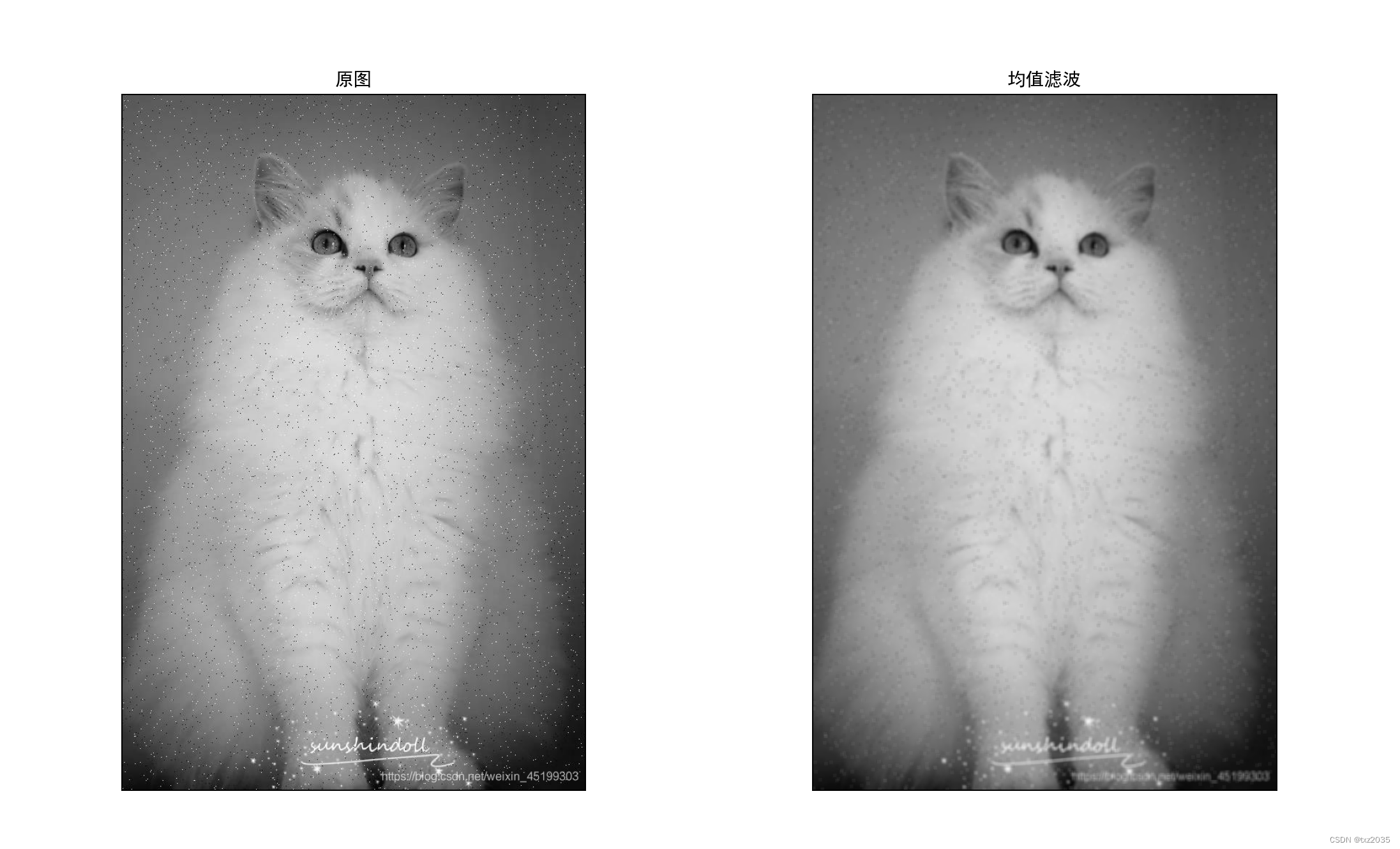
均值滤波
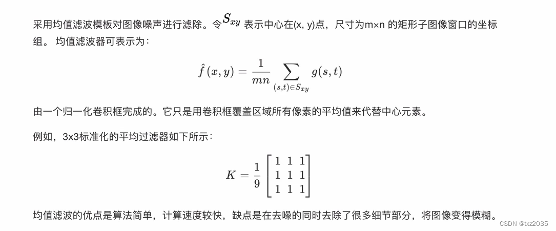

均值滤波代码实现
import cv2 as cv
import numpy as np
import matplotlib.pyplot as plt
from pylab import mpl

mpl.rcParams['font.sans-serif'] = ['SimHei']

img = cv.imread("dog.png")

#均值滤波
'''
cv.blur(img, (5, 5))将对图像img进行均值模糊处理。
参数(5, 5)表示卷积核的大小,这里是一个5x5的卷积核。卷积核的大小决定了模糊的程度,较大的卷积核会导致更强的模糊效果。
'''
blur = cv.blur(img,(5,5))

plt.figure(figsize=(5,4),dpi=100)
'''
plt.figure()函数用于创建一个新的图像窗口,并返回一个指向该窗口的引用。
figsize=(10, 8)参数指定了图像窗口的大小,这里设置为宽度为10英寸,高度为8英寸。
dpi=100参数指定了图像窗口的分辨率,这里设置为100。'''

plt.subplot(121),plt.imshow(img[:,:,::-1]),plt.title("原图")
'''
plt.subplot(121)函数用于创建一个子图区域。参数(121)表示将图像窗口分割为1行2列的网格,并选择第一个子图来显示图像。
plt.imshow(img[:, :, ::-1])函数用于显示图像。
img是需要显示的图像数组,[:, :, ::-1]表示对图像进行颜色通道的转换,由BGR顺序转换为RGB顺序。
plt.title("原图")函数用于设置子图的标题。
'''
plt.xticks([]),plt.yticks([])
'''
plt.xticks([])和plt.yticks([])函数用于设置坐标轴的刻度标签。
[]为空列表,表示不显示刻度标签,即去除x轴和y轴的刻度标签。
'''

plt.subplot(122),plt.imshow(blur[:,:,::-1]),plt.title("均值滤波")
plt.xticks([]),plt.yticks([])

plt.show()
结果展示
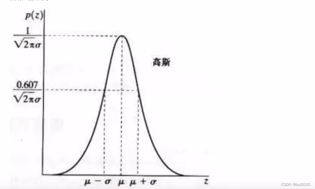
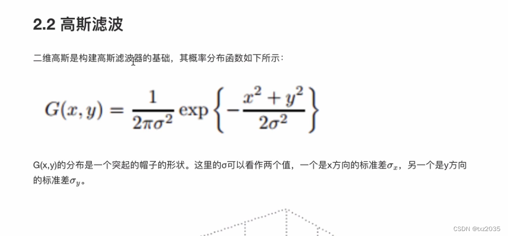
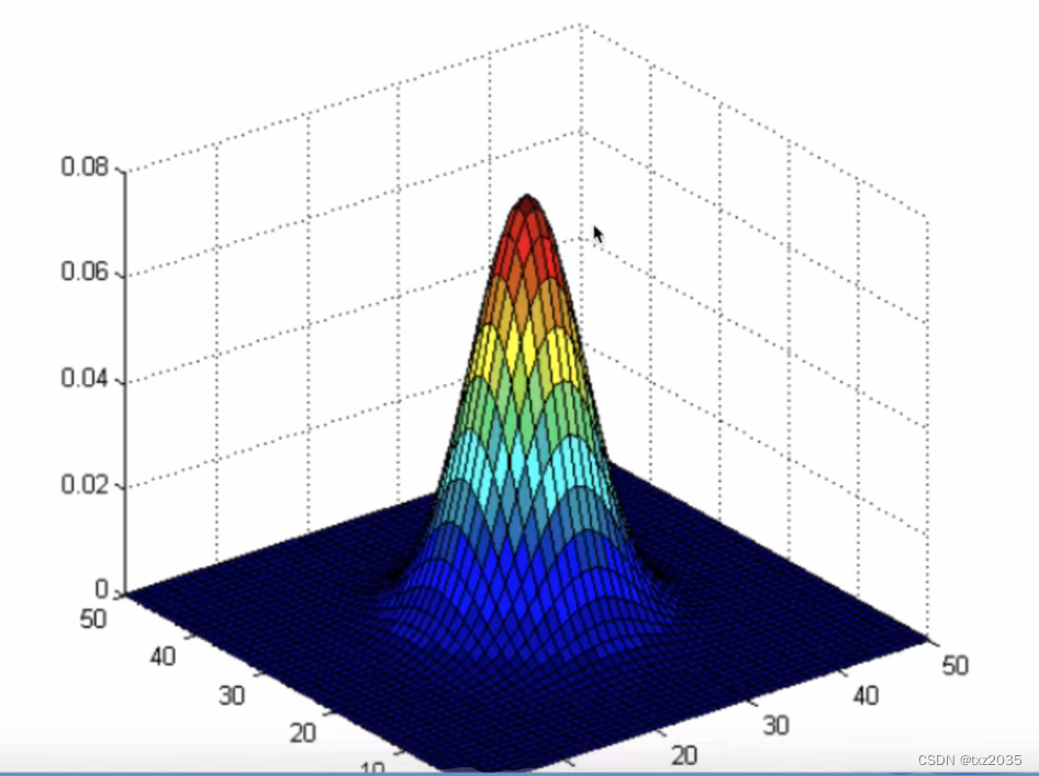
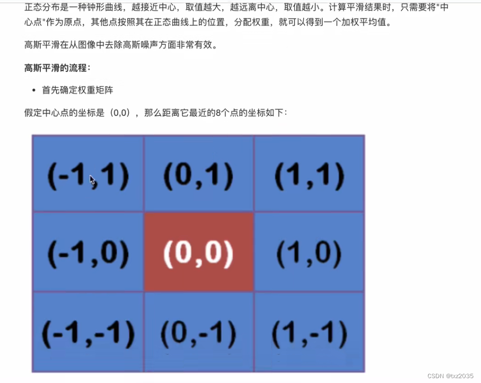
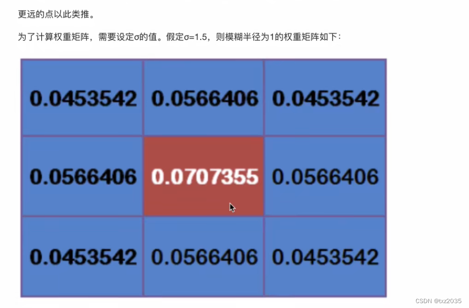
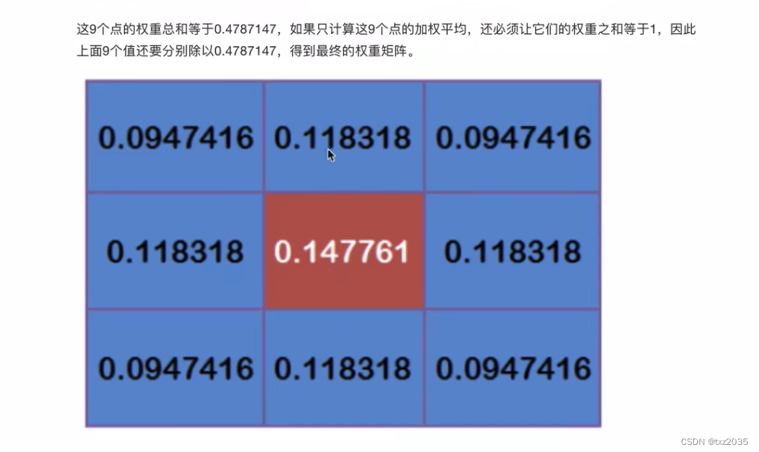
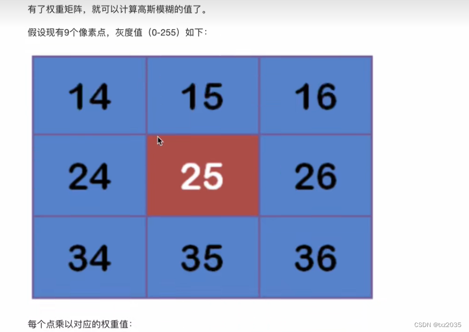
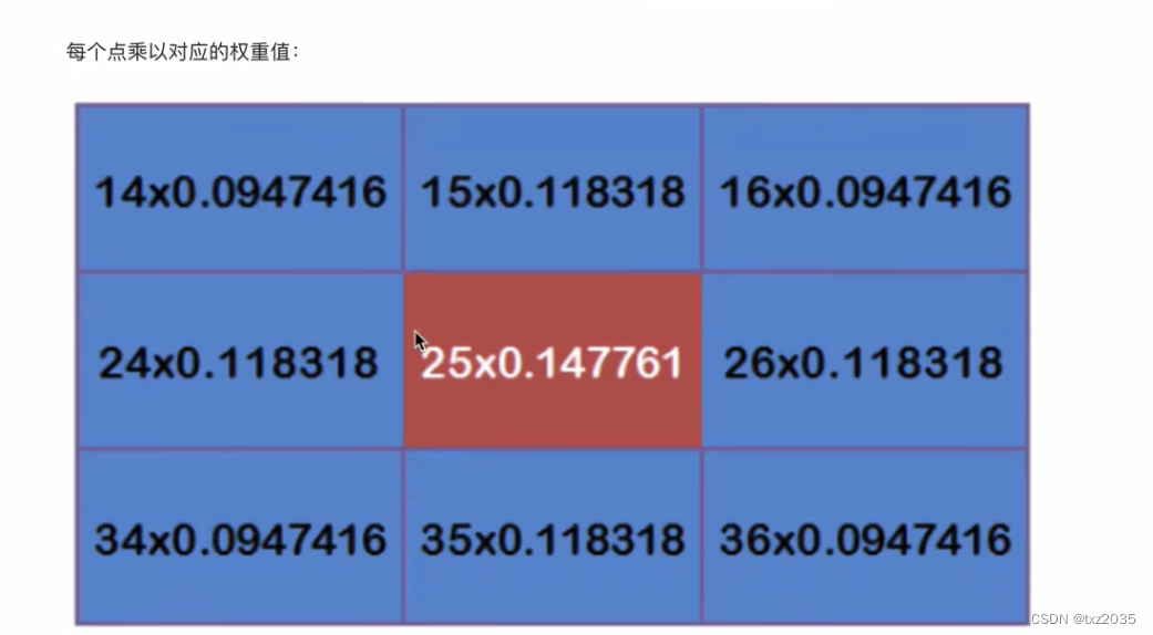
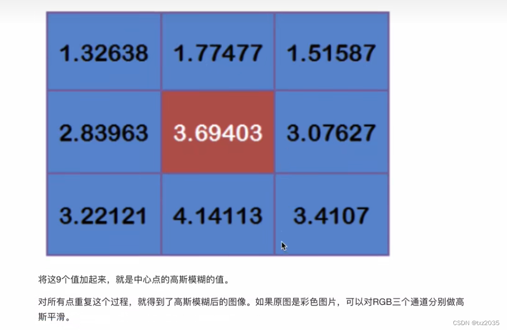
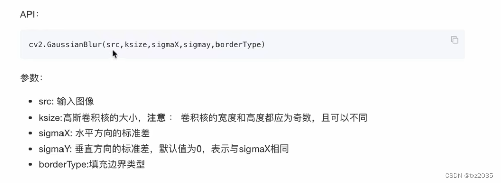
高斯滤波概念
代码实现
import cv2 as cv
import numpy as np
import matplotlib.pyplot as plt
from pylab import mpl
import random
mpl.rcParams['font.sans-serif'] = ['SimHei']
img =cv.imread("lena.png")
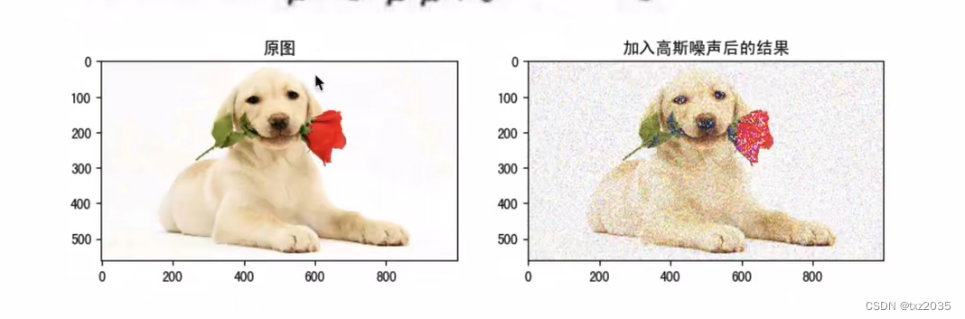
#添加高斯噪声
noise_sigma = 100 # 高斯噪声的标准差
noise = np.zeros(img.shape, np.int16)
cv.randn(noise, 0, noise_sigma)
img_with_noise = img + noise
img_with_noise = np.clip(img_with_noise, 0, 255).astype(np.uint8)
cv.imshow("Lena with Gaussian Noise", img_with_noise)
cv.waitKey(0)
blur = cv.GaussianBlur(img_with_noise,(3,3),1)
plt.figure(figsize=(5,4),dpi=100)
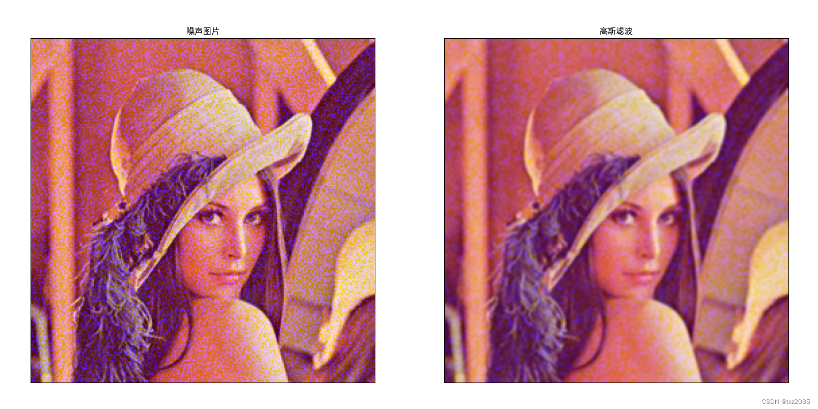
plt.subplot(121),plt.imshow(img_with_noise[:,:,::-1]),plt.title("噪声图片")
plt.xticks([]),plt.yticks([])
plt.subplot(122),plt.imshow(blur[:,:,::-1]),plt.title("高斯滤波")
plt.xticks([]),plt.yticks([])
plt.show()
结果展示
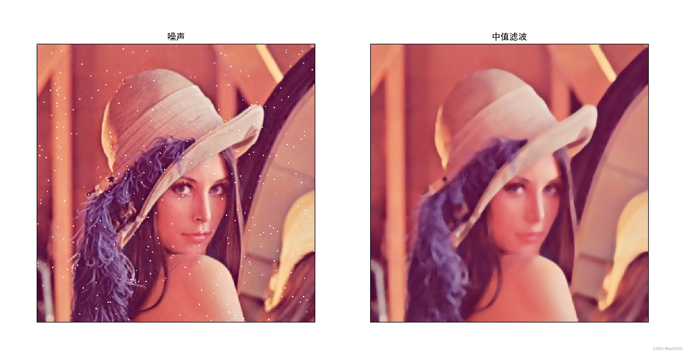
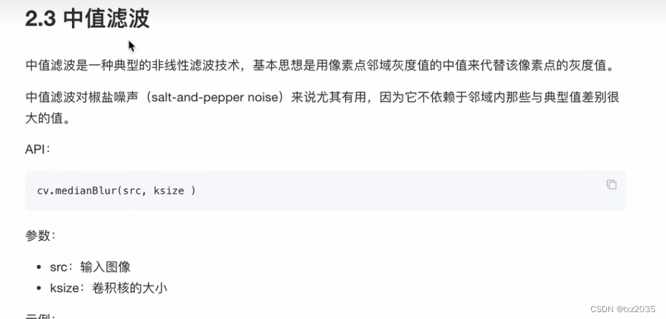
中值滤波
代码实现
import cv2 as cv
import numpy as np
import matplotlib.pyplot as plt
from pylab import mpl
import random

mpl.rcParams['font.sans-serif'] = ['SimHei']

img =cv.imread("lena.png")


#添加椒盐噪声
noise_density = 0.01  # 噪声比例

noise = np.zeros(img.shape[:2], np.uint8)

num_noise_pixels = int(noise_density * img.shape[0] * img.shape[1])

for _ in range(num_noise_pixels):
    x = random.randint(0, img.shape[1]-1)
    y = random.randint(0, img.shape[0]-1)
    if random.random() < 0.5:
        noise[y, x] = 0  # 设置为黑色
    else:
        noise[y, x] = 255  # 设置为白色

img_with_noise = cv.add(img, cv.cvtColor(noise, cv.COLOR_GRAY2BGR))

#中值滤波

blur = cv.medianBlur(img_with_noise,5)

#图像显示
plt.figure(figsize=(5,4),dpi=100)
plt.subplot(121),plt.imshow(img_with_noise[:,:,::-1]),plt.title("噪声")
plt.xticks([]),plt.yticks([])

plt.subplot(122),plt.imshow(blur[:,:,::-1]),plt.title("中值滤波")
plt.xticks([]),plt.yticks([])
plt.show()
结果展示