我不信中心极限定理

背景

在客观实际中有许多随机变量，它们是由大量的相互独立的随机因素的综合影响所形成的，而其中每一个别因素在总的影响中所起的作用都是微小的，这种随机变量往往近似地服从正态分布，这种现象就是中心极限定理。

由李雅普诺夫（Lyapunov）定理表示成公式形式就是：

设随机变量$X_1，X_2， ……，X_n，……$相互独立，它们具有数学期望和方差

$E(X_k)=μ_k，D(X_k)=σ^2_k，k=1，2，……$

记

$B^2_n=\sum^n_{k=1}σ^2_k$

当$n->∞$时

$\LARGE Z_n=\frac{\sum^n_{k=1}X_k-\sum^n_{k=1}μ_k}{B_n}∽N（0，1）$

这个定理表明，无论各个随机变量$X_k，（k=1，2，……）$服从什么分布，只要满足定理的条件，那么它们的和$\sum^n_{k=1}X_k$当$n$很大时，就近似地服从正态分布。

---

疑问

多个随机变量分布不同，期望不同，方差不同，仅仅单凭数量足够多和相互独立这两个条件，就可以断定它们的和近似服从正态分布吗？数学理论推导方面我不是专家，但是仅仅简单的定理证明却不能让我信服，下面我将通过程序的方式对随机变量进行模拟，测试多个不同的随机变量之和是否服从正态分布，以及对它们的期望，方差的估计值，定理是否准确。

---

随机变量分布的生成模拟

这里选取8种常见的随机变量，对其分布进行模拟生成。选取的分布依次为，零一分布，二项分布，帕斯卡分布，几何分布，超几何分布，泊松分布，均匀分布，正态分布。全部源代码实现ProbabilityFunctions.py参见附录。

基本每一种分布都包含以下两个方法：

• 一个根据指定参数生成一个符合当前分布的值的方法
• 一个生成指定数量的满足指定分布但是参数随机的方法

下面分别对每一种模拟的实现进行简单介绍。

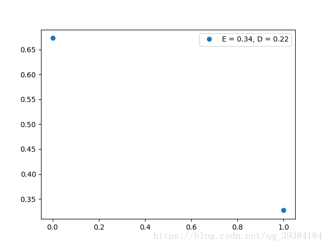
零一分布

ZeroOneDistribution方法根据参数p，根据分布生成一个随机的值，而randomZOD方法根据参数Cnt，随机生成Cnt个满足零一分布的值，而零一分布的参数也是随机的，最后返回生成的值，期望和方差。

根据randomZOD方法生成的分布函数测试如下：

源代码实现：

def ZeroOneDistribution(p):
 if p > np.random.rand():
  result = 1
 else:
  result = 0
 return result, p, p*(1-p)

def randomZOD(Cnt = 1):
 p = np.random.rand()
 data = []
 tmp = ZeroOneDistribution(p)
 data.append(tmp[0])
 for i in range(1, Cnt):
  data.append(ZeroOneDistribution(p)[0])
 return data, tmp[1], tmp[2]

---

二项分布

二项分布实际为n次零一分布的总和，因此方法类似，这里不再给出详细解释。

但是由于解决数值较大导致计算时产生溢出的问题，这里设置二项分布的参数n的范围为（10，100）。

根据randomTED方法生成的分布函数测试如下：

源代码实现：

TED_Max_N = 100
TED_Min_N = 10

def TwoEntryDistribution(n, p):
 result = 0
 for i in range(n):
  if p > np.random.rand():
   result += 1
 return result, n*p, n*p*(1-p)

def randomTED(Cnt = 1):
 n = np.random.randint(TED_Min_N, TED_Max_N)
 p = np.random.rand()
 data = []
 tmp = TwoEntryDistribution(n, p)
 data.append(tmp[0])
 for i in range(1, Cnt):
  data.append(TwoEntryDistribution(n, p)[0])
 return data, tmp[1], tmp[2]

---

帕斯卡分布

帕斯卡分布与零一分布也有一定的相似之处，表示为r次成功的次数，因此有两个参数r和p。程序实现中使用了一个while循环，当成功次数达到r次时则返回总共的实验次数n。

同样的，为了防止溢出，设置帕斯卡分布的参数r的范围为（10，100）。

根据randomPaD方法生成的分布函数测试如下：

源代码实现：

PaD_Max_R = 100
PaD_Min_R = 10

def PascalDistribution(r, p):
 result = 0
 winNum = 0
 while(winNum < r):
  if p > np.random.rand():
   winNum += 1
  result += 1
 return result, r/p, r*(1-p)/p/p

def randomPaD(Cnt = 1):
 r = np.random.randint(PaD_Min_R, PaD_Max_R)
 p = np.random.rand()
 data = []
 tmp = PascalDistribution(r, p)
 data.append(tmp[0])
 for i in range(1, Cnt):
  data.append(PascalDistribution(r, p)[0])
 return data, tmp[1], tmp[2]

---

几何分布

几何分布是帕斯卡分布r=1时的特殊形式。

根据randomGD方法生成的分布函数测试如下：

源代码实现：

def GeometricDistribution(p):
 return PascalDistribution(1, p)

def randomGD(Cnt = 1):
 p = np.random.rand()
 data = []
 tmp = GeometricDistribution(p)
 data.append(tmp[0])
 for i in range(1, Cnt):
  data.append(GeometricDistribution(p)[0])
 return data, tmp[1], tmp[2]

---

超几何分布

超几何分布虽然与几何分布名字相近，但是分布却完全不一样。超几何分布可以简单表示为总共N件样品，其中有M件次品$（M<N）$，从中随机抽取n件样品，其中次品的个数。因此超几何分布有3个参数N，M，n。程序实现中使用了一个0到n的for循环，根据随机数来判断是否选中次品，并且抽中次品后N和M的值都要减一，如果没有抽中次品则只有N减一，最后返回总共抽取的次品数目。

同样的，为了防止溢出，设置超几何分布的参数N的范围为（10，100）。

根据randomHGD方法生成的分布函数测试如下：

源代码实现：

HGD_Max_N = 100
HGD_Min_N = 10

def HypergeometricDistribution(N, M, n):
 result = 0
 E = n*M/N
 D = E*(1-M/N)*(N-n)/(N-1)
 for i in range(n):
  if M > np.random.randint(N):
   M -= 1
   result += 1
  N -= 1
 return result, E, D

def randomHGD(Cnt = 1):
 N = np.random.randint(HGD_Min_N, HGD_Max_N)
 M = np.random.randint(N)
 n = np.random.randint(2, N)
 data = []
 tmp = HypergeometricDistribution(N, M, n)
 data.append(tmp[0])
 for i in range(1, Cnt):
  data.append(HypergeometricDistribution(N, M, n)[0])
 return data, tmp[1], tmp[2]

---

泊松分布

泊松分布是二项分布的n很大，p很小时的一种近似情况，由于泊松分布的迭代计算比较麻烦，所以采用查表的方式来进行泊松分布的计算。具体实现思路如下：首先设置PoissonDistributionTable函数，当Poisson_Distribution_Table.txt不存在的时候先创建泊松分布表，计算出所有需要的泊松分布对应λ值和x值的概率，之后在进行泊松分布的计算时只需要查表即可。这里需要到的λ值的范围为arange(0.1, 1, 0.1)，arange(1, 10, 0.5)和np.arange(10, 19, 1)，为常用的泊松分布的λ值的范围

根据randomHGD方法生成的分布函数测试如下：

源代码实现：

Po_Lambda_Arange = np.append(np.arange(0.1, 1, 0.1), np.arange(1, 10, 0.5))
Po_Lambda_Arange = np.append(Po_Lambda_Arange, np.arange(10, 19, 1))

def PoissonDistributionTable():
 f = open('Poisson_Distribution_Table.txt', 'w')
 for Lambda in Po_Lambda_Arange:
  k = 0
  paiK = 1
  p = np.power(Lambda, k)*np.power(np.e, -Lambda)/paiK
  f.write(str(round(p, 6)) + ' ')
  while abs(p - 1.0) > EPSILON:
   k += 1
   paiK *= k
   pTmp = np.power(Lambda, k)*np.power(np.e, -Lambda)/paiK
   p += pTmp
   f.write(str(round(p, 6)) + ' ')
  f.write('1.000000')
  f.write('\n')
 f.close()

def PoissonDistribution(Lambda):
 try:
  f = open('Poisson_Distribution_Table.txt')
 except FileNotFoundError:
  PoissonDistributionTable()
  f = open('Poisson_Distribution_Table.txt')
 index = np.argwhere(Po_Lambda_Arange == Lambda)
 for v in f:
  index -= 1
  if index == -1:
   distributions = v
   break
 f.close()
 distributions = np.array(list(map(float, distributions.split("\n")[0].split(" "))))
 results = np.argwhere(distributions < np.random.rand())
 result = len(results)
 return result, Lambda, Lambda

def randomPoD(Cnt = 1):
 Lambda = np.random.choice(Po_Lambda_Arange)
 data = []
 tmp = PoissonDistribution(Lambda)
 data.append(tmp[0])
 for i in range(1, Cnt):
  data.append(PoissonDistribution(Lambda)[0])
 return data, tmp[1], tmp[2]

---

均匀分布

均匀分布是一种连续的分布，为了计算和绘图的方便，在返回样本值的时候将其强制转换为整形。均匀分布有两个参数a和b，返回值在（a，b）之间的概率是等值的，但是由于程序取整的原因，在a值处的概率实际为在（a，a+0.4）范围内的概率，而中间值c处的概率实际为在（c-0.4，c+0.4）范围内的概率，所以端点值的概率为中间值的二分之一，但是并不影响之后的模拟。

同样的，为了防止溢出，设置超几何分布的参数a和b的范围为（-100，100）。并选取较大值为a，较小值为b。

根据randomUD方法生成的分布函数测试如下：

源代码实现：

UD_Max = 100
UD_Min = -100

def UniformDstribution(a, b):
 result = np.random.rand()*(b-a)+a
 E = (a+b)/2
 D = np.power(b-a, 2)/12
 return int(round(result)), E, D

def randomUD(Cnt = 1):
 a = np.random.randint(UD_Min, UD_Max)
 b = np.random.randint(UD_Min, UD_Max)
 if a > b:
  a = a^b
  b = a^b
  a = a^b
 data = []
 tmp = UniformDstribution(a, b)
 data.append(tmp[0])
 for i in range(1, Cnt):
  data.append(UniformDstribution(a, b)[0])
 return data, tmp[1], tmp[2]

---

正态分布

正态分布的值模拟直接采用读正态分布表的方式实现，根据随机生成的值去正态分布表中读取对应的分布值，正态分布表提前加载到了Normal_Distribution_Table.txt里，格式为：每向下一行，分布值增加0.1，每向右一列，分布值增加0.01，如果分布概率小于0.5，即分布值为负，则先计算对应的正值，最后在转化为负值，正态分布表参见文末附录。

正态分布的生成函数除了期望，方差两个参数之外，还有一个默认参数p，为正态分布的概率，默认随机生成，但也可以给定参数由ND方法绘制均匀的正态分布图像。

同样的，为了防止溢出，设置正态分布的期望的范围为（-100，100），方差的范围为（0，100）。

根据randomND方法生成的分布函数测试如下：

根据ND方法生成的分布函数测试如下：

源代码实现：

ND_Max_E = 100
ND_Min_E = -100
ND_Max_D = 100

def NormalDistribution(E, D, p = -1):
 if p == -1:
  p = np.random.rand()
 f = open('Normal_Distribution_Table.txt')
 if p > 0.5:
  positive = True
 else:
  p = 1 - p
  positive = False
 i = 0
 for v in f:
  j = 0
  v = np.array(list(map(float, v.split("\n")[0].split(" "))))
  for k in v:
   if k > p:
    f.close()
    result = i+j
    if not positive:
     result = -result
    result = result*np.sqrt(D)+E
    return int(result), E, D
   j += 0.01
  i += 0.1
 f.close()
 if positive:
  result = 3
 else:
  result = -3
 result = result*np.sqrt(D)+E
 return int(result), E, D

def randomND(Cnt = 1):
 E = np.random.randint(ND_Min_E,ND_Max_E)
 D = np.random.randint(ND_Max_D)
 data = []
 tmp = NormalDistribution(E, D)
 data.append(tmp[0])
 for i in range(1, Cnt):
  data.append(NormalDistribution(E, D)[0])
 return data, tmp[1], tmp[2]

def ND(E, D):
 data = []
 tmp = NormalDistribution(E, D, 0)
 data.append(tmp[0])
 for p in np.arange(0.0001, 1.0000, 0.0001):
  data.append(NormalDistribution(E, D, p)[0])
 return data, tmp[1], tmp[2]

随机分布

由于验证中心极限定理需要随机分布的随机变量，所以这里添加一个通用的函数，根据随机生成的值选择8中随机变量中的一种并返回，源代码实现如下：

def random(Cnt = 1):
 index = np.random.randint(8)
 if index == 0:
  return randomZOD(Cnt)
 elif index == 1:
  return randomTED(Cnt)
 elif index == 2:
  return randomPaD(Cnt) 
 elif index == 3:
  return randomGD(Cnt)  
 elif index == 4:
  return randomHGD(Cnt) 
 elif index == 5:
  return randomPoD(Cnt) 
 elif index == 6:
  return randomUD(Cnt) 
 else:
  return randomND(Cnt)

分布图绘制处理

分布图绘制处理分为三部分。

一，数据处理

参数为随机的数据样本和作图取样点步长，返回作图的X，Y值数组和坐标轴范围。

首先默认的作图取样点数目为100，所以默认的取样点步长为取样点总数除以100；X值为数据的最小值到最大值的范围，Y值为指定步长内数据点的数量，最后在除以总数作标准化，以使总概率和为1；坐标轴X轴范围为数据的最小值到最大值的范围，Y轴范围为0到概率最大值的1.2倍。

二，绘制指定的正态分布图像便于后续比较*

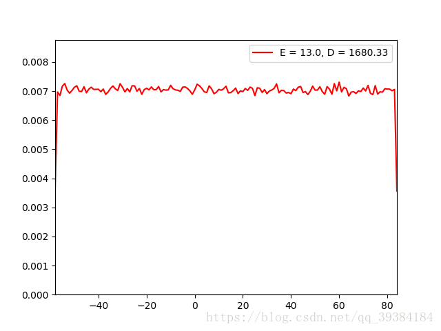
使用上面的ND函数得到均匀的正态分布数据，由测试得到在默认的10000个数据点的前提下，步长为3时可以绘制到最合适的正态分布图像。

三，主函数

根据传入的参数：分布类型，计算取样点数目（默认为1000），作图取样点步长：（默认为计算取样点数目/100）和是否开启坐标轴适配（均匀分布建议开启）得到相应的分布图像，当然，虽然分布已知，但是分布的参数确实随机的。运行截图如下：

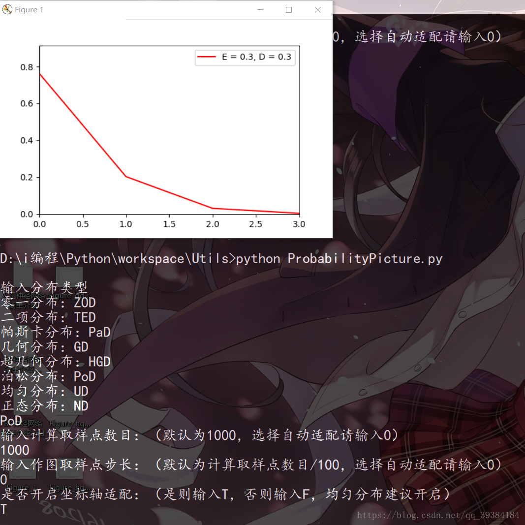
源代码实现ProbabilityPicture.py参见附录：

---

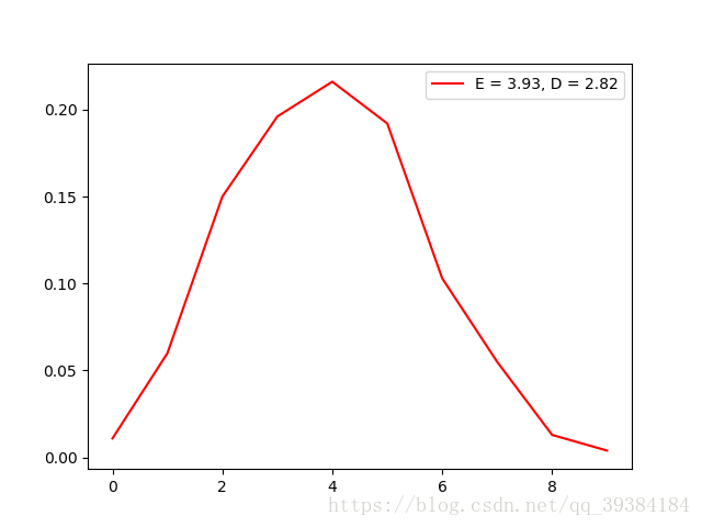
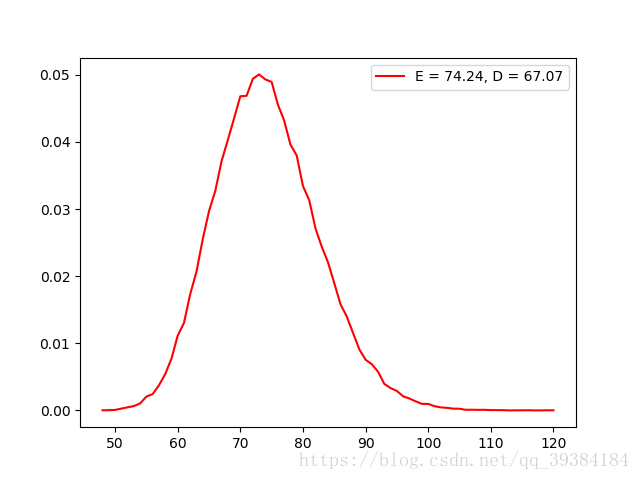
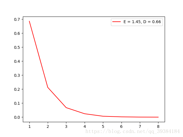
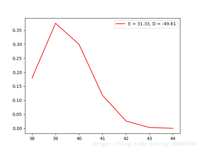
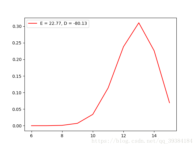
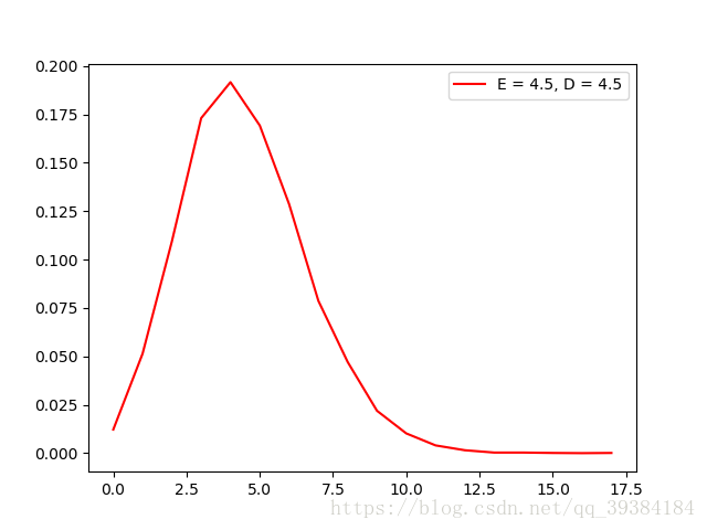
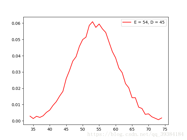
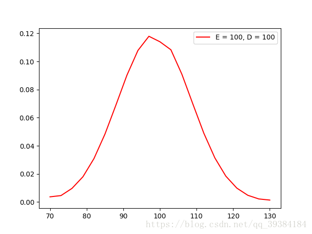
观察多个随机变量之和的分布图

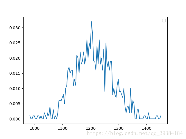
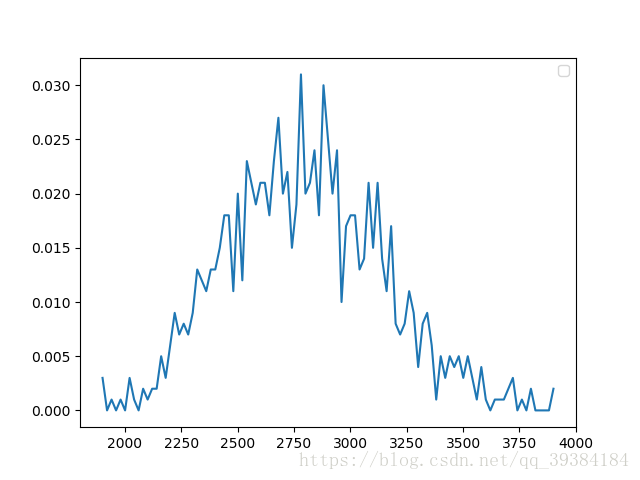
前面的8种随机变量测试完毕之后，通过调用random方法来生成随机的分布，测试10个，25个，50个随机变量生成的分布图如下：

10个随机变量

25个随机变量

50个随机变量

这里选取计算取样次数为1000次，绘图取样点为100，通过改变N的值来改变变量的数目。

源代码示例：

from ProbabilityFunctions import *
from ProbabilityPicture import *
import numpy as np
import matplotlib.pyplot as plt

Cnt = 1000# 取样次数
N = 10# 变量数目
E = 0# 总期望
D = 0# 总方差
Data = [0]*Cnt

Data = np.array(Data)

for i in range(N):
 print(i)
 dataTmp, eTmp, dTmp = random(Cnt)
 E += eTmp
 D += dTmp
 Data += dataTmp

X, Y, Axis = OperateData(Data)

plt.plot(X, Y, '-')
plt.legend()
plt.show()

通过对分布图的观察，还不能简单的判断它是否符合分布，不仅需要对其进行分布假设检验，还需要求其期望和方差的置信区间。下面是对本文采取的分布拟合检验方法和求期望和方差的置信区间的方法的介绍。

---

分布拟合检验

这是对随机变量是否服从正态分布的一种检验方法，虽然卡方拟合检验法是检验总体分布的较一般的方法，但用它来检验总体的正态性时，犯第二类错误的概率往往较大，为此统计学家对检验正态分布的种种方法进行了比较，认为“偏度，峰度检验法”及“夏皮罗——威尔克法”较为有效。这里采用的是偏度，峰度检验法。

理论介绍

随机变量X的偏度和峰度指的是X的标准化变量$\LARGE \frac{X-E(X)}{\sqrt{D(X)}}$的三阶矩和四阶矩：

$\LARGE ν_1=E[(\frac{X-E(X)}{\sqrt{D(X)}})^3]=\frac{E[(X-E(X))^3]}{(D(X))^{\frac{3}{2}}}$

$\LARGE ν_2=E[(\frac{X-E(X)}{\sqrt{D(X)}})^4]=\frac{E[(X-E(X))^4]}{(D(X))^2}$

当随机变量服从正态分布时，$ν_1=0$且$ν_2=3$。

设$X_1，X_2， ……，X_n$是来自总体X的样本，则$ν_1，ν_2$的矩估计量分别是：

$\LARGE G_1=\frac{B_3}{B^{\frac{3}{2}}_2}$

$\LARGE G_2=\frac{B_4}{B^2_2}$

其中$B_k（2，3，4）$是样本k阶中心矩，并分别称$G_1，G_2$为样本偏度和样本峰度。

若总体X为正态变量，则可证明当n充分大时，近似有：

$\LARGE G_1∽N（0，\frac{6(n-2)}{(n+1)(n+3)}）$

$\LARGE G_2∽N（3-\frac{6}{n+1}，\frac{24n(n-2)(n-3)}{(n+1)^2(n+3)(n+5)}）$

设$X_1，X_2， ……，X_n$是来自总体X的样本，现在来检验假设

$H_0$：X是正态总体。

记

$σ_1=\sqrt{\frac{6(n-2)}{(n+1)(n+3)}}，σ_2=\sqrt{\frac{24n(n-2)(n-3)}{(n+1)^2(n+3)(n+5)}}$

$μ_2=3-\frac{6}{n+1}，U_1=\frac{G_1}{σ_1}，U_2=\frac{G_2-μ_2}{α_2}$

当$H_0$为真且n充分大时，近似地有：

$U_1∽N（0，1），U_2∽N（0，1）$

取显著性水平为α，$H_0$的拒绝域为：

$|u_1|≥k_1或|u_2|≥k_2$

由

$P\{当H_0为真拒绝H_0\}$

$=P_{H_0}\{（|U_1|≥z_{α/4}）∪（|U_2|≥z_{α/4}）\}$

$≤P_{H_0}\{|U_1|≥z_{α/4}\}+P_{H_0}\{|U_2|≥z_{α/4}\}$

$=\frac{α}{2}+\frac{α}{2}=α$

得拒绝域为

$|u_1|≥z_{α/4}或|u_2|≥z_{α/4}$

---

函数实现

由于程序比较简单，这里不再给出详细说明，只是点出几个要点。

• 参数为被检验样本值的数组，返回值为表示是否服从正态分布的布尔值
• 选取显著性水平为0.1，预定义全局变量Z_alpha_0_025 = 1.96
• EXPECT方法计算样本期望，CENTER方法计算样本的中心矩，函数源代码参见附录ProbabilityMain.py
• 由于测试选取的随机变量数量繁多，因此高阶中心矩的计算如果超过64位程序最大实数的范围则返回“warning”，而此函数返回”longlong overflow”。
• 程序源代码如下

def JudgeNormal(data):
 n = len(data)
 A1 = EXPECT(data)
 A2 = CENTER(data, 2)
 A3 = CENTER(data, 3)
 A4 = CENTER(data, 4)
 if A1 == "waring" or A2 == "waring" or A3 == "waring" or A4 == "waring":
  print("longlong overflow")
  return "longlong overflow"
 sigma1 = np.sqrt(6*(n-2)/(n+1)/(n+3))
 sigma2 = np.sqrt(24*n*(n-2)*(n-3)/(n+1)/(n+1)/(n+3)/(n+5))
 mu2 = 3-6/(n+1)
 B2 = A2 - np.power(A1, 2)
 B3 = A3 - 3*A2*A1 + 2*np.power(A1, 3)
 B4 = A4 - 4*A3*A1 + 6*A2*np.power(A1, 2) - 3*np.power(A1, 4)
 g1 = B3/np.power(B2, 1.5)
 g2 = B4/np.power(B2, 2)
 u1 = abs(g1/sigma1)
 u2 = abs(g2-mu2)/sigma2
 return u1 < Z_alpha_0_025 and u2 < Z_alpha_0_025

---

期望的方差的置信区间

期望

由方差未知的情况下的期望置信区间公式。

$\LARGE （X^-±\frac{S}{\sqrt{n}}t_{α/2}(n-1)）$

这里选取显著性水平为0.05；而由于测试选取的样本数量非常多，远大于100，所以这里的t分位点近似等于z分位点；SAMPLE_VARIANCE方法计算样本方差，函数源代码参见附录ProbabilityMain.py。

源代码实现：

# 样本均值置信区间，alpha = 0.05
def CONFIDENCE_EXPECT(data):
 k = SAMPLE_VARIANCE(data)
 k = np.sqrt(k)
 n = len(data)
 k = k/np.sqrt(n)*Z_alpha_0_025
 E = EXPECT(data)
 return round(E-k,2), round(E+k,2)

---

方差

由期望未知的情况下的方差的置信区间公式。

$\LARGE （\frac{(n-1)S^2}{X^2_{α/2}(n-1)}，\frac{(n-1)S^2}{X^2_{1-α/2}(n-1)}）$

这里选取显著性水平为0.05；而由于测试选取的样本数量非常多，远大于40，由卡方分位点的计算公式：

$当n>40时，X^2_α(n)≈\frac{1}{2}(z_α+\sqrt{2n-1})^2$

所以根据z分位点和n值来计算卡方分位点；SAMPLE_VARIANCE方法计算样本方差，函数源代码参见附录ProbabilityMain.py。

源代码实现：

# 样本方差置信区间，alpha = 0.05
def CONFIDENCE_VARIANCE(data):
 n = len(data)
 k = SAMPLE_VARIANCE(data)*(n-1)
 Chi_alpha_0_025 = Chi_alpha(Z_alpha_0_025, n)
 Chi_alpha_0_975 = Chi_alpha(-Z_alpha_0_025, n)
 return round(k/Chi_alpha_0_025,2), round(k/Chi_alpha_0_975,2)

---

中心极限定理的验证

正态分布的验证

下面依次选取N在range（5，50）范围内的值，进行分布拟合检验，每个N值计算10次，最后求一个服从正态分布的概率。值得注意的是，由于存在longlong溢出的问题，无法简单的将其消除，只能尽可能避免，下面所采取到的策略是：若发生longlong溢出，则抛弃此次计算的数据值，重新选取分布，直到有10个有效数据值为止。

示例输出如下：

n=5 p=0.6
n=6 p=0.9
n=7 p=1.0
n=8 p=0.9
n=9 p=1.0
n=10 p=0.8
n=11 p=0.7
n=12 p=0.8
n=13 p=0.8
n=14 p=0.8
n=15 p=0.8
n=16 p=0.7
n=17 p=0.9
n=18 p=0.8
n=19 p=0.9
n=20 p=0.6
n=21 p=1.0
n=22 p=0.9
n=23 p=0.9
n=24 p=0.9
n=25 p=0.9
n=26 p=0.8
n=27 p=0.8
n=28 p=0.8
n=29 p=0.9
n=30 p=0.8
n=31 p=1.0
n=32 p=1.0
n=33 p=0.6
n=34 p=0.9
n=36 p=0.9
n=38 p=0.9
n=39 p=0.7
n=40 p=0.7
n=41 p=0.6
n=42 p=0.9
n=43 p=1.0
n=44 p=0.8
n=45 p=0.9
n=46 p=1.0
n=47 p=0.8
n=48 p=0.9
n=49 p=0.5
n=50 p=0.9

可以看出，当N增大时，分布以大约一个0.9的概率符合正态分布。所以近似的，可以将N>25时的分布看做符合正态分布。

源代码示例：

from ProbabilityFunctions import *
from ProbabilityPicture import *
import numpy as np

if __name__ == '__main__':
 Cnt = 100# 取样次数
 N = 50# 变量数目

 # 输出预测结果
 import sys

 output = sys.stdout
 outputfile = open('ProbabilityResult.txt', 'w')
 sys.stdout = outputfile
 for n in range(5, 50):
  N = n
  results = []
  while len(results) < 10:

   E = 0# 总期望
   D = 0# 总方差
   Data = [0]*Cnt

   Data = np.array(Data)

   for i in range(N):
    dataTmp, eTmp, dTmp = random(Cnt)
    E += eTmp
    D += dTmp
    Data += dataTmp

   result = JudgeNormal(Data)
   if result == "longlong overflow":
    continue
   results.append(result)
   print(len(results))
   outputfile.flush()
  p = results.count(True)
  p = p/len(results)
  print('n='+str(n)+' p='+str(p))
 outputfile.close()
 sys.stdout = output

---

期望和方差的值的验证

下面选取N为50，取样次数为1000时，分别使用中心极限定理的公式和最大似然估计法求其期望的方差，再使用上面介绍的方法求其期望和方差的置信区间。

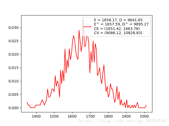
可以看出，最大似然法估计的期望和方差与中心极限定理公式中给出的计算值相近，而且其值也完全包含在置信区间内。

源代码示例：

Cnt = 1000# 取样次数
N = 50# 变量数目
E = 0# 总期望
D = 0# 总方差
Data = [0]*Cnt

Data = np.array(Data)

for i in range(N):
 print(i)
 dataTmp, eTmp, dTmp = random(Cnt)
 E += eTmp
 D += dTmp
 Data += dataTmp

X, Y, Axis = OperateData(Data)

CE = CONFIDENCE_EXPECT(Data)
CV = CONFIDENCE_VARIANCE(Data)

msg = 'E = ' + str(round(E, 2))+', D = ' + str(round(D, 2))+'\nE^ = ' + str(round(EXPECT(Data), 2))+', D^ = ' + str(round(VARIANCE(Data), 2))+'\nCE = ' + str(CE)+'\nCV = ' + str(CV)

plt.plot(X, Y, 'r', label = msg)
plt.legend()
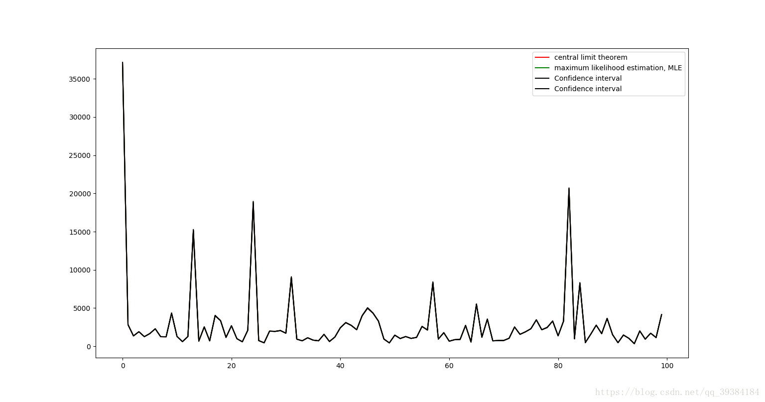
plt.show()

下面分别计算100次的结果并进行绘图处理。图像中包括中心极限定理计算出的理论值，由最大似然法计算出来的估计值，和由置信区间计算出来的上下限。100次的结果绘制成曲线绘制如下：

期望图

方差图

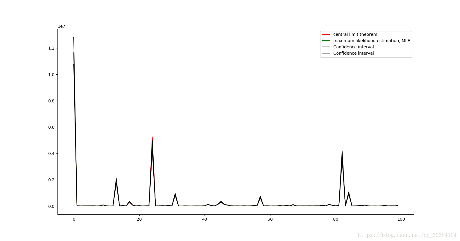
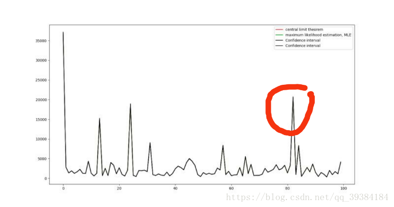
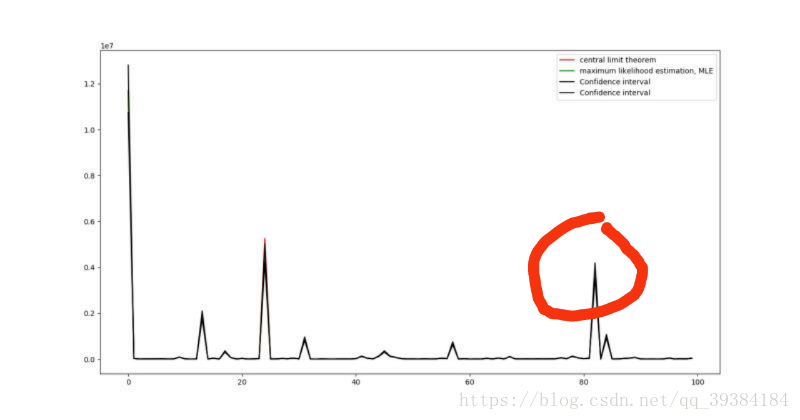
图像中红线表示中心极限定理计算出的理论值，绿线表示由最大似然法计算出来的估计值，黑线由置信区间计算出来的上下限，由于4个值及其接近，所以我们放大红色圆圈部分如下图所示：

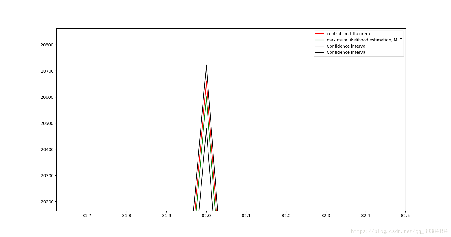
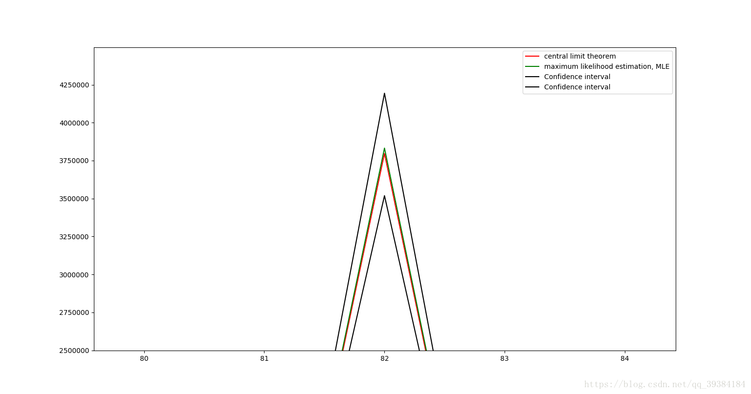
可以看出，由中心极限定理计算出来的期望值和方差值是非常准确的。

源代码示例：

from ProbabilityFunctions import *
from ProbabilityPicture import *
import numpy as np
import matplotlib.pyplot as plt

EList = []
DList = []
EEList = []
DDList = []
CEList = []
CVList = []

for count in range(100):
 Cnt = 1000# 取样次数
 N = 50# 变量数目
 E = 0# 总期望
 D = 0# 总方差
 Data = [0]*Cnt

 Data = np.array(Data)

 for i in range(N):
  print(i)
  dataTmp, eTmp, dTmp = random(Cnt)
  E += eTmp
  D += dTmp
  Data += dataTmp


 CE = CONFIDENCE_EXPECT(Data)
 CV = CONFIDENCE_VARIANCE(Data)

 EE = EXPECT(Data)
 DD = VARIANCE(Data)

 EList.append(E)
 DList.append(D)
 EEList.append(EE)
 DDList.append(DD)
 CEList.append(CE)
 CVList.append(CV)

X = range(100)

CEUP = []
CEDOEN = []

for i in range(len(CEList)):
 CEUP.append(CEList[i][0])
 CEDOEN.append(CEList[i][1])

CVUP = []
CVDOEN = []

for i in range(len(CVList)):
 CVUP.append(CVList[i][0])
 CVDOEN.append(CVList[i][1])

plt.plot(X, EList, 'r', label = 'central limit theorem')
plt.plot(X, EEList, 'g', label = 'maximum likelihood estimation, MLE')
plt.plot(X, CEUP, 'black', label = 'Confidence interval')
plt.plot(X, CEDOEN, 'black', label = 'Confidence interval')
plt.legend()
plt.show()

plt.plot(X, DList, 'r', label = 'central limit theorem')
plt.plot(X, DDList, 'g', label = 'maximum likelihood estimation, MLE')
plt.plot(X, CVUP, 'black', label = 'Confidence interval')
plt.plot(X, CVDOEN, 'black', label = 'Confidence interval')
plt.legend()
plt.show()

---

应用

中心极限定理是正态随机变量在概率论中占有重要地位的一个基本原因，在很多问题中，所考虑的随机变量可以表示成很多个独立的随机变量之和。例如，在任一指定时刻，一个城市的耗电量是大量用户耗电量的总和；一个物理实验的测量误差是由许多观察不到的，可加的微小误差所合成的，但是它们往往都近似地服从正态分布，所以可以使用正态分布的性质进行相关的预测，模拟和计算。

---

附录1：Normal_Distribution_Table.txt

0.5000 0.5040 0.5080 0.5120 0.5160 0.5199 0.5239 0.5279 0.5319 0.5359
0.5398 0.5438 0.5478 0.5517 0.5557 0.5596 0.5636 0.5675 0.5714 0.5753
0.5793 0.5832 0.5871 0.5910 0.5948 0.5987 0.6026 0.6064 0.6103 0.6141
0.6179 0.6217 0.6255 0.6293 0.6331 0.6368 0.6406 0.6443 0.6480 0.6517
0.6554 0.6591 0.6628 0.6664 0.6700 0.6736 0.6772 0.6808 0.6844 0.6879
0.6915 0.6950 0.6985 0.7019 0.7054 0.7088 0.7123 0.7157 0.7190 0.7224
0.7257 0.7291 0.7324 0.7357 0.7389 0.7422 0.7454 0.7486 0.7517 0.7549
0.7580 0.7611 0.7642 0.7673 0.7703 0.7734 0.7764 0.7794 0.7823 0.7582
0.7881 0.7910 0.7939 0.7967 0.7995 0.8023 0.8051 0.8078 0.8106 0.8133
0.8159 0.8186 0.8212 0.8238 0.8264 0.8289 0.8315 0.8340 0.8365 0.8389
0.8413 0.8438 0.8461 0.8485 0.8508 0.8531 0.8554 0.8577 0.8599 0.8621
0.8643 0.8665 0.8686 0.8708 0.8729 0.8749 0.8770 0.8790 0.8810 0.8830
0.8849 0.8869 0.8888 0.8907 0.8925 0.8944 0.8962 0.8980 0.8997 0.9015
0.9032 0.9049 0.9066 0.9082 0.9099 0.9115 0.9131 0.9147 0.9162 0.9177
0.9192 0.9207 0.9222 0.9236 0.9251 0.9265 0.9278 0.9292 0.9306 0.9319
0.9332 0.9345 0.9357 0.9370 0.9382 0.9394 0.9406 0.9418 0.9430 0.9441
0.9452 0.9463 0.9474 0.9484 0.9495 0.9505 0.9515 0.9525 0.9535 0.9545
0.9554 0.9564 0.9573 0.9582 0.9591 0.9599 0.9608 0.9616 0.9625 0.9633
0.9641 0.9648 0.9656 0.9664 0.9671 0.9678 0.9686 0.9693 0.9700 0.9706
0.9713 0.9719 0.9726 0.9732 0.9738 0.9744 0.9750 0.9756 0.9762 0.9767
0.9772 0.9778 0.9783 0.9788 0.9793 0.9798 0.9803 0.9808 0.9812 0.9817
0.9821 0.9826 0.9830 0.9834 0.9838 0.9842 0.9846 0.9850 0.9854 0.9857
0.9861 0.9864 0.9868 0.9871 0.9874 0.9878 0.9881 0.9884 0.9887 0.9890
0.9893 0.9896 0.9898 0.9901 0.9904 0.9906 0.9909 0.9911 0.9913 0.9916
0.9918 0.9920 0.9922 0.9925 0.9927 0.9929 0.9931 0.9932 0.9934 0.9936
0.9938 0.9940 0.9941 0.9943 0.9945 0.9946 0.9948 0.9949 0.9951 0.9952
0.9953 0.9955 0.9956 0.9957 0.9959 0.9960 0.9961 0.9962 0.9963 0.9964
0.9965 0.9966 0.9967 0.9968 0.9969 0.9970 0.9971 0.9972 0.9973 0.9974
0.9974 0.9975 0.9976 0.9977 0.9977 0.9978 0.9979 0.9979 0.9980 0.9981
0.9981 0.9982 0.9982 0.9983 0.9984 0.9984 0.9985 0.9985 0.9986 0.9986

---

附录2：ProbabilityFunctions.py

import numpy as np

EPSILON = 0.00001
TED_Max_N = 100
TED_Min_N = 10
PaD_Max_R = 100
PaD_Min_R = 10
HGD_Max_N = 100
HGD_Min_N = 10
Po_Lambda_Arange = np.append(np.arange(0.1, 1, 0.1), np.arange(1, 10, 0.5))
Po_Lambda_Arange = np.append(Po_Lambda_Arange, np.arange(10, 19, 1))
UD_Max = 100
UD_Min = -100
ND_Max_E = 100
ND_Min_E = -100
ND_Max_D = 100


def ZeroOneDistribution(p):
 if p > np.random.rand():
  result = 1
 else:
  result = 0
 return result, p, p*(1-p)

def randomZOD(Cnt = 1):
 p = np.random.rand()
 data = []
 tmp = ZeroOneDistribution(p)
 data.append(tmp[0])
 for i in range(1, Cnt):
  data.append(ZeroOneDistribution(p)[0])
 return data, tmp[1], tmp[2]

def TwoEntryDistribution(n, p):
 result = 0
 for i in range(n):
  if p > np.random.rand():
   result += 1
 return result, n*p, n*p*(1-p)

def randomTED(Cnt = 1):
 n = np.random.randint(TED_Min_N, TED_Max_N)
 p = np.random.rand()
 data = []
 tmp = TwoEntryDistribution(n, p)
 data.append(tmp[0])
 for i in range(1, Cnt):
  data.append(TwoEntryDistribution(n, p)[0])
 return data, tmp[1], tmp[2]

def PascalDistribution(r, p):
 result = 0
 winNum = 0
 while(winNum < r):
  if p > np.random.rand():
   winNum += 1
  result += 1
 return result, r/p, r*(1-p)/p/p

def randomPaD(Cnt = 1):
 r = np.random.randint(PaD_Min_R, PaD_Max_R)
 p = np.random.rand()
 data = []
 tmp = PascalDistribution(r, p)
 data.append(tmp[0])
 for i in range(1, Cnt):
  data.append(PascalDistribution(r, p)[0])
 return data, tmp[1], tmp[2]

def GeometricDistribution(p):
 return PascalDistribution(1, p)

def randomGD(Cnt = 1):
 p = np.random.rand()
 data = []
 tmp = GeometricDistribution(p)
 data.append(tmp[0])
 for i in range(1, Cnt):
  data.append(GeometricDistribution(p)[0])
 return data, tmp[1], tmp[2]

def HypergeometricDistribution(N, M, n):
 result = 0
 E = n*M/N
 D = E*(1-M/N)*(N-n)/(N-1)
 for i in range(n):
  if M > np.random.randint(N):
   M -= 1
   result += 1
  N -= 1
 return result, E, D

def randomHGD(Cnt = 1):
 N = np.random.randint(HGD_Min_N, HGD_Max_N)
 M = np.random.randint(N)
 n = np.random.randint(2, N)
 data = []
 tmp = HypergeometricDistribution(N, M, n)
 data.append(tmp[0])
 for i in range(1, Cnt):
  data.append(HypergeometricDistribution(N, M, n)[0])
 return data, tmp[1], tmp[2]

def PoissonDistributionTable():
 f = open('Poisson_Distribution_Table.txt', 'w')
 for Lambda in Po_Lambda_Arange:
  k = 0
  paiK = 1
  p = np.power(Lambda, k)*np.power(np.e, -Lambda)/paiK
  f.write(str(round(p, 6)) + ' ')
  while abs(p - 1.0) > EPSILON:
   k += 1
   paiK *= k
   pTmp = np.power(Lambda, k)*np.power(np.e, -Lambda)/paiK
   p += pTmp
   f.write(str(round(p, 6)) + ' ')
  f.write('1.000000')
  f.write('\n')
 f.close()

def PoissonDistribution(Lambda):
 try:
  f = open('Poisson_Distribution_Table.txt')
 except FileNotFoundError:
  PoissonDistributionTable()
  f = open('Poisson_Distribution_Table.txt')
 index = np.argwhere(Po_Lambda_Arange == Lambda)
 for v in f:
  index -= 1
  if index == -1:
   distributions = v
   break
 f.close()
 distributions = np.array(list(map(float, distributions.split("\n")[0].split(" "))))
 results = np.argwhere(distributions < np.random.rand())
 result = len(results)
 return result, Lambda, Lambda

def randomPoD(Cnt = 1):
 Lambda = np.random.choice(Po_Lambda_Arange)
 data = []
 tmp = PoissonDistribution(Lambda)
 data.append(tmp[0])
 for i in range(1, Cnt):
  data.append(PoissonDistribution(Lambda)[0])
 return data, tmp[1], tmp[2]

def UniformDstribution(a, b):
 result = np.random.rand()*(b-a)+a
 E = (a+b)/2
 D = np.power(b-a, 2)/12
 return int(round(result)), E, D

def randomUD(Cnt = 1):
 a = np.random.randint(UD_Min, UD_Max)
 b = np.random.randint(UD_Min, UD_Max)
 if a > b:
  a = a^b
  b = a^b
  a = a^b
 data = []
 tmp = UniformDstribution(a, b)
 data.append(tmp[0])
 for i in range(1, Cnt):
  data.append(UniformDstribution(a, b)[0])
 return data, tmp[1], tmp[2]

def NormalDistribution(E, D, p = -1):
 if p == -1:
  p = np.random.rand()
 f = open('Normal_Distribution_Table.txt')
 if p > 0.5:
  positive = True
 else:
  p = 1 - p
  positive = False
 i = 0
 for v in f:
  j = 0
  v = np.array(list(map(float, v.split("\n")[0].split(" "))))
  for k in v:
   if k > p:
    f.close()
    result = i+j
    if not positive:
     result = -result
    result = result*np.sqrt(D)+E
    return int(result), E, D
   j += 0.01
  i += 0.1
 f.close()
 if positive:
  result = 3
 else:
  result = -3
 result = result*np.sqrt(D)+E
 return int(result), E, D

def randomND(Cnt = 1):
 E = np.random.randint(ND_Min_E,ND_Max_E)
 D = np.random.randint(ND_Max_D)
 data = []
 tmp = NormalDistribution(E, D)
 data.append(tmp[0])
 for i in range(1, Cnt):
  data.append(NormalDistribution(E, D)[0])
 return data, tmp[1], tmp[2]

def ND(E, D):
 data = []
 tmp = NormalDistribution(E, D, 0)
 data.append(tmp[0])
 for p in np.arange(0.0001, 1.0000, 0.0001):
  data.append(NormalDistribution(E, D, p)[0])
 return data, tmp[1], tmp[2]

def random(Cnt = 1):
 index = np.random.randint(8)
 if index == 0:
  return randomZOD(Cnt)
 elif index == 1:
  return randomTED(Cnt)
 elif index == 2:
  return randomPaD(Cnt) 
 elif index == 3:
  return randomGD(Cnt)  
 elif index == 4:
  return randomHGD(Cnt) 
 elif index == 5:
  return randomPoD(Cnt) 
 elif index == 6:
  return randomUD(Cnt) 
 else:
  return randomND(Cnt)

---

附录3：ProbabilityPicture.py

from ProbabilityFunctions import *
import matplotlib.pyplot as plt

DrawPointCnt = 100# 作图取样点数目
Cnt = 1000# 计算取样点数目
delta = 0# 作图取样步长

def OperateData(data, delta = 0):
 Xmin = min(data)
 Xmax = max(data)
 data = list(data)
 Y = []

 # delta为作图取样步长
 if delta == 0:
  delta = int((Xmax-Xmin)/DrawPointCnt)
 if delta == 0:
  delta = 1

 for i in range(Xmin, Xmax+1, delta):
  Y.append(data.count(i))
  for j in range(i+1, i+delta):
   Y[len(Y)-1] += data.count(j)

 # 标准化：使概率和为1
 sumY = sum(Y)
 for i in range(len(Y)):
  Y[i] = Y[i]/sumY

 X = range(Xmin, Xmax+1, delta)
 Axis = (Xmin, Xmax, 0, (max(Y)*1.2))
 return X, Y, Axis

def drawND(E, D):
 Data, E, D = ND(E, D)
 X, Y, Axis = OperateData(Data,3)
 plt.plot(X, Y, 'g', label = msg)

if __name__ == '__main__':
 # 运行命令
 # python ProbabilityPicture.py

 # 替换函数名称来生成不同的分布图像

 Distribution = input('''
输入分布类型
零一分布：ZOD
二项分布：TED
帕斯卡分布：PaD
几何分布：GD
超几何分布：HGD
泊松分布：PoD
均匀分布：UD
正态分布：ND
''')
 Cnt = int(input('输入计算取样点数目：（默认为1000，选择自动适配请输入0）\n'))
 if Cnt == 0:
  Cnt = 1000
 delta = int(input('输入作图取样点步长：（默认为计算取样点数目/100，选择自动适配请输入0）\n'))
 if Distribution == 'ZOD':
  Data, E, D = randomZOD(Cnt)
 elif Distribution == 'TED':
  Data, E, D = randomTED(Cnt)
 elif Distribution == 'PaD':
  Data, E, D = randomPaD(Cnt)
 elif Distribution == 'GD':
  Data, E, D = randomGD(Cnt)
 elif Distribution == 'HGD':
  Data, E, D = randomHGD(Cnt)
 elif Distribution == 'PoD':
  Data, E, D = randomPoD(Cnt)
 elif Distribution == 'UD':
  Data, E, D = randomUD(Cnt)
 elif Distribution == 'ND':
  Data, E, D = randomND(Cnt)
 else:
  print("Input Error")

 X, Y, Axis = OperateData(Data, delta)

 msg = 'E = ' + str(round(E, 2))+', D = ' + str(round(D, 2))

 bo = input('是否开启坐标轴适配：（是则输入T，否则输入F，均匀分布建议开启）\n')

 if bo == 'T':
  plt.axis(Axis)

 plt.plot(X, Y, 'r', label = msg)
 plt.legend()
 plt.show()

---

附录4：ProbabilityMain.py

from ProbabilityFunctions import *
from ProbabilityPicture import *
import numpy as np
import matplotlib.pyplot as plt

Z_alpha_0_025 = 1.96
LongLongMax = 1<<63

def Chi_alpha(Z_alpha, n):
 Chi = Z_alpha + np.sqrt(2*n-1)
 Chi = np.power(Chi, 2)
 Chi = Chi/2
 return Chi

def EXPECT(data):
 sumd = np.longlong(0)
 for d in data:
  sumd += d
 return sumd/len(data)

def CENTER(data, pow):
 sumd = np.longlong(0)
 for d in data:
  dd = np.longlong(d)
  for i in range(pow-1):
   if d != 0 and LongLongMax / d < dd:
    print("warning")
    return "waring"
   dd = dd*d
  if LongLongMax - sumd < dd:
   print("warning")
   return "waring"
  sumd = sumd + dd
 return sumd/len(data)

def VARIANCE(data):
 EX = EXPECT(data)
 data = np.power(data-EX, 2)
 return EXPECT(data)

def SAMPLE_VARIANCE(data):
 n = len(data)
 d = VARIANCE(data)
 return d*n/(n-1)

# 样本均值置信区间，alpha = 0.05
def CONFIDENCE_EXPECT(data):
 k = SAMPLE_VARIANCE(data)
 k = np.sqrt(k)
 n = len(data)
 k = k/np.sqrt(n)*Z_alpha_0_025
 E = EXPECT(data)
 return round(E-k,2), round(E+k,2)

# 样本方差置信区间，alpha = 0.05
def CONFIDENCE_VARIANCE(data):
 n = len(data)
 k = SAMPLE_VARIANCE(data)*(n-1)
 Chi_alpha_0_025 = Chi_alpha(Z_alpha_0_025, n)
 Chi_alpha_0_975 = Chi_alpha(-Z_alpha_0_025, n)
 return round(k/Chi_alpha_0_025,2), round(k/Chi_alpha_0_975,2)

'''
test_data = [
141,148,132,138,154,142,150,146,155,158,150,140,147,148,144,150,149,145,149,158,143,141,144,144,126,140,144,142,141,140,145,135,147,146,141,136,140,146,142,137,148,154,137,139,143,140,131,143,141,149,148,135,148,152,143,144,141,143,147,146,150,132,142,142,143,153,149,146,149,138,142,149,142,137,134,144,146,147,140,142,140,137,152,145]
test_A1 = 143.7738
test_A2 = 20706.13
test_A3 = 2987099
test_A4 = 4.316426E8
test_B2 = 35.2246
test_B3 = -28.5
test_B4 = 3840
test_sigma1 = 0.2579
test_sigma2 = 0.4892
test_mu2 = 2.9294
test_g1 = -0.1363
test_g2 = 3.0948
test_u1 = 0.5285
test_u2 = 0.3381
'''

# 检验是否为正态分布, alpha = 0.1
def JudgeNormal(data):
 n = len(data)
 A1 = EXPECT(data)
 A2 = CENTER(data, 2)
 A3 = CENTER(data, 3)
 A4 = CENTER(data, 4)
 if A1 == "waring" or A2 == "waring" or A3 == "waring" or A4 == "waring":
  print("longlong overflow")
  return "longlong overflow"
 sigma1 = np.sqrt(6*(n-2)/(n+1)/(n+3))
 sigma2 = np.sqrt(24*n*(n-2)*(n-3)/(n+1)/(n+1)/(n+3)/(n+5))
 mu2 = 3-6/(n+1)
 B2 = A2 - np.power(A1, 2)
 B3 = A3 - 3*A2*A1 + 2*np.power(A1, 3)
 B4 = A4 - 4*A3*A1 + 6*A2*np.power(A1, 2) - 3*np.power(A1, 4)
 g1 = B3/np.power(B2, 1.5)
 g2 = B4/np.power(B2, 2)
 u1 = abs(g1/sigma1)
 u2 = abs(g2-mu2)/sigma2
 return u1 < Z_alpha_0_025 and u2 < Z_alpha_0_025

# 运行命令
# python ProbabilityMain.py

if __name__ == '__main__':
 Cnt = 100# 取样次数
 N = 50# 变量数目

 # 输出预测结果
 import sys

 output = sys.stdout
 outputfile = open('ProbabilityResult.txt', 'w')
 sys.stdout = outputfile
 for n in range(5, 50):
  N = n
  results = []
  while len(results) < 10:

   E = 0# 总期望
   D = 0# 总方差
   Data = [0]*Cnt

   Data = np.array(Data)

   for i in range(N):
    dataTmp, eTmp, dTmp = random(Cnt)
    E += eTmp
    D += dTmp
    Data += dataTmp

   result = JudgeNormal(Data)
   if result == "longlong overflow":
    continue
   results.append(result)
   print(len(results))
   outputfile.flush()
  p = results.count(True)
  p = p/len(results)
  print('n='+str(n)+' p='+str(p))
 outputfile.close()
 sys.stdout = output


'''
Cnt = 1000# 取样次数
N = 50# 变量数目
E = 0# 总期望
D = 0# 总方差
Data = [0]*Cnt

Data = np.array(Data)

for i in range(N):
 print(i)
 dataTmp, eTmp, dTmp = random(Cnt)
 E += eTmp
 D += dTmp
 Data += dataTmp

X, Y, Axis = OperateData(Data)

CE = CONFIDENCE_EXPECT(Data)
CV = CONFIDENCE_VARIANCE(Data)

msg = 'E = ' + str(round(E, 2))+', D = ' + str(round(D, 2))+'\nE^ = ' + str(round(EXPECT(Data), 2))+', D^ = ' + str(round(VARIANCE(Data), 2))+'\nCE = ' + str(CE)+'\nCV = ' + str(CV)

plt.plot(X, Y, 'r', label = msg)
plt.legend()
plt.show()
'''

'''
Cnt = 1000# 取样次数
N = 10# 变量数目
E = 0# 总期望
D = 0# 总方差
Data = [0]*Cnt

Data = np.array(Data)

for i in range(N):
 print(i)
 dataTmp, eTmp, dTmp = random(Cnt)
 E += eTmp
 D += dTmp
 Data += dataTmp

X, Y, Axis = OperateData(Data)

plt.plot(X, Y, '-')
plt.legend()
plt.show()
'''

'''
EList = []
DList = []
EEList = []
DDList = []
CEList = []
CVList = []

for count in range(100):
 Cnt = 1000# 取样次数
 N = 50# 变量数目
 E = 0# 总期望
 D = 0# 总方差
 Data = [0]*Cnt

 Data = np.array(Data)

 for i in range(N):
  print(i)
  dataTmp, eTmp, dTmp = random(Cnt)
  E += eTmp
  D += dTmp
  Data += dataTmp


 CE = CONFIDENCE_EXPECT(Data)
 CV = CONFIDENCE_VARIANCE(Data)

 EE = EXPECT(Data)
 DD = VARIANCE(Data)

 EList.append(E)
 DList.append(D)
 EEList.append(EE)
 DDList.append(DD)
 CEList.append(CE)
 CVList.append(CV)

X = range(100)

CEUP = []
CEDOEN = []

for i in range(len(CEList)):
 CEUP.append(CEList[i][0])
 CEDOEN.append(CEList[i][1])

CVUP = []
CVDOEN = []

for i in range(len(CVList)):
 CVUP.append(CVList[i][0])
 CVDOEN.append(CVList[i][1])

plt.plot(X, EList, 'r', label = 'central limit theorem')
plt.plot(X, EEList, 'g', label = 'maximum likelihood estimation, MLE')
plt.plot(X, CEUP, 'black', label = 'Confidence interval')
plt.plot(X, CEDOEN, 'black', label = 'Confidence interval')
plt.legend()
plt.show()

plt.plot(X, DList, 'r', label = 'central limit theorem')
plt.plot(X, DDList, 'g', label = 'maximum likelihood estimation, MLE')
plt.plot(X, CVUP, 'black', label = 'Confidence interval')
plt.plot(X, CVDOEN, 'black', label = 'Confidence interval')
plt.legend()
plt.show()
'''