Autoencoder:机器学习中的自动编码器,这篇文章里面用的是去噪编码器,坊间称之为denoise autoencoder(DAE),在sc-RNAseq中除去dropout的噪声是非常理想的一种模型。
Therefore,这篇文章已经发表在了NC的18年预印本上,证明其方法和文章质量很是不错。
基本原理of DAE:
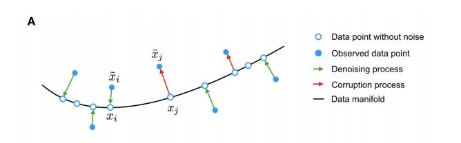
###measurement noise from dropout events, moves data points away from the data manifold (black line). The autoencoder is trained to denoise the data by mapping corrupted data points back onto the data manifold (green arrows),蓝色实心点代表的是corruption points(变体位点)也就是被观测到的点,而蓝色空心点代表的是没有noise的数据点。而manifold则是指的是流形学习中形成的分类流。manifold learning也是一种非常常用以及常见的机器学习方法,后续中我们依然会进一步的介绍。
而文章中,说明的是DCA takes the count distribution(数目分布), overdispersion and sparsity of the data(过离散性和稀疏性) into account using a zero-inflated negative binomial noise model(零膨胀负二项模型,后续会对ZINB模型做进一步的介绍,因为本puppy对它很是钟爱), and nonlinear gene-gene(基因与基因之间的非线性作用) or gene-dispersion (基因与离散度的交互作用)interactions are captured.
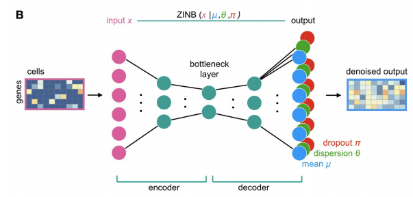
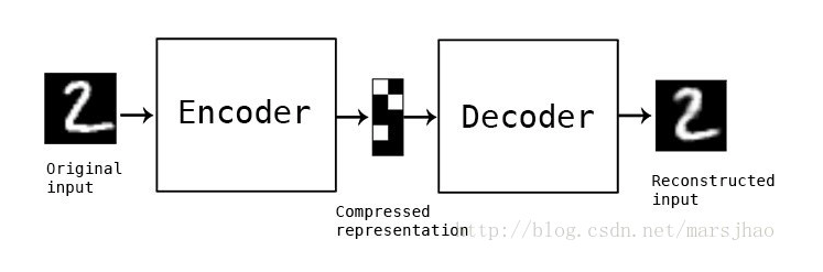
Input counts, mean, dispersion and dropout probabilities are denoted as x, μ, θ and π. respectively。A typical autoencoders compresses high dimensional data into lower dimensions in order to constrain the model and extract features that summarize the data well in the bottleneck layer.
Extension in machine learning:
###################
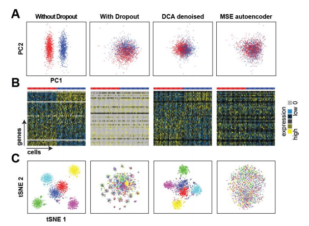
To test whether a ZINB loss function is necessary, we compared DCA to a classical autoencoder with mean squared error (MSE) loss function using log transformed count data. The MSE based autoencoder was unable to recover the celltypes, indicating that the specialized ZINB loss function is necessary for scRNA-seq data.
下述为没有dp的数据,有dp的数据,DCA的ZINB损失函数的的去噪自动编码器method,以及经典DCA中log化之后的均方误的损失函数method。主要目的是突出它们开发的新型零膨胀负二项分布的损失函数的模型优越性,是显著优于经典函数的模型。四种情况下的分类,降维以及聚类分析印证。文中很多显示该法优越性的图,本文重方法,画图这里不多表。
method:
ZINB is parameterized with mean and dispersion parameters of the negative binomial component (μ and θ) and the mixture coefficient that represents the weight of the point mass (π):这里的派指的是dropout基因表达量计数的权重——estimates dropout
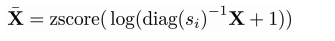
首先,调整基因表达矩阵的library size, log value 以及 z-score normalization
再用Xbar 去计算E B D分别代表的是编码层,瓶颈层以及解码层的不同matrix
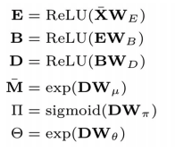
前三步在进行矩阵的LU分解
后三步在根据分解出来的矩阵进行参数的定义,D是解码层得出的激活函数矩阵
The loss function that is likelihood of zero-inflated negative binomial distribution:
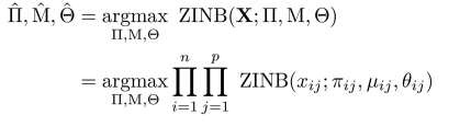
根据上述系列等式得到的参数,损失函数的参数估计,其中的估计过程就用到了ZINB分布,其中的M代表的是乘上了size factor的mean matrix,公式如: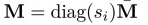
同时,如果你有不同的dp rate的权重,你就需要不同用dp以及零膨胀参数的脊先验概率去估计它:公式如下:
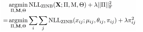
where NLLZINB function represents the negative log likelihood of ZINB distribution.
||TT||^2是TT在二维空间向量中的范数大小。使用ZINB的负逻辑似然值去估计X TT M 塞塔变得可行。
而范数是线性代数以及机器学习中矢量空间中的重要概念:
范数,是具有“长度”概念的函数。在泛函分析以及线性代数及相关的数学领域,范数是一个函数,是矢量空间内的所有矢量赋予非零的正长度或大小。半范数可以为非零的矢量赋予零长度。它常常被用来度量某个向量空间(或矩阵)中的每个向量的长度或大小。
总之,这个公式的优点在于可以在不同量级或者等级的基因离散程度上都有很好的参数估计效果。(cites:the alternative option estimates a scalar dispersion parameter per gene )
====================================
====================================
现存的很多单细胞优化的分析软件有:scImpute、MAGIC、DCA、SAVER、BEIR、etc
大家感兴趣的可以去搜索一下,以飨the socpe your knowledge
