Inception层中,有多个卷积层结构(Conv)和Pooling结构(MaxPooling),它们利用padding原理,经过这些结构的最终结果shape不变。
一、Inception的基础概念
Inception模块在GoogLeNet中首次提出并采用,其基本结构如下图所示,带有1X1卷积核的Inception层,就构成了Inception网络的基本单元,整个inception结构就是由多个这样的inception模块串联起来的。Inception网络对输入图像进行并行采集特征,并将所有输出结果拼接为一个非常深的特征图,由于并行提取特征时卷积核大小不一样,这在一定程度上丰富了特征,使特征多样化。同时并行采集信号特征的方式,使每一层都能学到不同特征,既增加了网络的宽度,又增加了网络对尺度的适应性。
二、Inception构造基础单元
Inception典型构造之一:

用pytorch实现模型构造:
# 2. 设计基础模型
class InceptionA(torch.nn.Module):
    def __init__(self, inChannels):                                 # inChannels表输入通道数
        super(InceptionA, self).__init__()
        # 2.1 第一层池化 + 1*1卷积
        self.branch1_1x1 = nn.Conv2d(in_channels=inChannels,  # 输入通道
                                           out_channels=24,         # 输出通道
                                           kernel_size=1)           # 卷积核大小1*1
        # 2.2 第二层1*1卷积
        self.branch2_1x1 = nn.Conv2d(inChannels, 16, kernel_size=1)

        # 2.3 第三层
        self.branch3_1_1x1 = nn.Conv2d(inChannels, 16, kernel_size=1)
        self.branch3_2_5x5 = nn.Conv2d(16, 24, kernel_size=5, padding=2)
        # padding=2,因为要保持输出的宽高保持一致

        # 2.4 第四层
        self.branch4_1_1x1 = nn.Conv2d(inChannels, 16, kernel_size=1)
        self.branch4_2_3x3 = nn.Conv2d(16, 24, kernel_size=3, padding=1)
        self.branch4_3_3x3 = nn.Conv2d(24, 24, kernel_size=3, padding=1)

    def forward(self, X_input):
        # 第一层
        branch1_pool = F.avg_pool2d(X_input,        # 输入
                                    kernel_size=3,  # 池化层的核大小3*3
                                    stride=1,       # 每次移动一步
                                    padding=1)
        branch1 = self.branch1_1x1(branch1_pool)
        # 第二层
        branch2 = self.branch2_1x1(X_input)
        # 第三层
        branch3_1= self.branch3_1_1x1(X_input)
        branch3 = self.branch3_2_5x5(branch3_1)
        # 第四层
        branch4_1 = self.branch4_1_1x1(X_input)
        branch4_2 = self.branch4_2_3x3(branch4_1)
        branch4 = self.branch4_3_3x3(branch4_2)
        # 输出
        output = [branch2, branch3, branch4, branch1]
        # (batch_size, channel, w, h)   dim=1: 即安装通道进行拼接。
        # eg: (1, 2, 3, 4) 和 (1, 4, 3, 4)按照dim=1拼接,则拼接后的shape为(1, 2+4, 3,  4)
        return torch.cat(output, dim=1)
三、1*1卷积核加入的原因
为什么要这样设计?
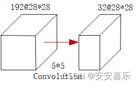
如下图所示,一个输入的张量,它有192个通道,图像大小为28*28,当我们用5*5做卷积的时候,那么卷积所用的浮点运算就是这样的一个值:5^2× 28^2× 192× 32=120,422,400。
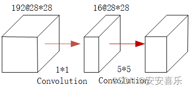
如果我们加上一个1*1的卷积,变成下图的样子,它实际的运算量就是:1^2 ×28^2 ×192 ×16+5^2× 28^2×16 × 32=12,433,648。通过卷积改变通道数,看似结构复杂,但是运算量却大大减少。使用1X1的卷积核实现了降维操作,以此来减少网络的参数量。
总结:Inception结构的主要贡献有两个:一是使用1x1的卷积来进行升降维;二是在多个尺寸上同时进行卷积再聚合。对于现在的卷积神经网络来说,提升网络性能最保险的方法就是增加网络的宽度和深度,这样做同时也会伴随着副作用。第一个副作用表现为越深越宽的网络往往会意味着有巨大的参数量,当数据量很少的时候,训练出来的网络很容易过拟合,第二个副作用表现在当网络有很深的深度的时候,很容易造成梯度消失现象。这两个副作用制约着又深又宽的卷积神经网络的发展,Inception网络很好的解决了这两个问题。
四、pytorch实现(采用的使MNIST数据集)
import torch
import torch.nn as nn
import torchvision.utils
from torchvision import transforms
from torchvision import datasets
from torch.utils.data import DataLoader
import torch.nn.functional as F
import torch.optim as optim
import matplotlib.pyplot as plt
import time

# 1.数据准备
batch_size = 64
transform = transforms.Compose([transforms.ToTensor(), transforms.Normalize((0.1307,), (0.3081,))])
# 做归一化和放长

# 1.1: 加载数据
train_dataset = datasets.MNIST(root='../dataset/mnist/',    # 获取数据
                               train=True,                  # 表示获取数据集
                               download=True,               # 若本地没有,则下载
                               transform=transform)
# 1.2: 按照batch_size划分成小样本
train_loader = DataLoader(dataset=train_dataset,
                          shuffle=True,
                          batch_size=batch_size)

test_dataset = datasets.MNIST(root='../dataset/mnist/', train=False, download=True, transform=transform)
test_loader = DataLoader(dataset=test_dataset, shuffle=True, batch_size=batch_size)

# 2. 设计基础模型
class InceptionA(torch.nn.Module):
    def __init__(self, inChannels):                                 # inChannels表输入通道数
        super(InceptionA, self).__init__()
        # 2.1 第一层池化 + 1*1卷积
        self.branch1_1x1 = nn.Conv2d(in_channels=inChannels,  # 输入通道
                                           out_channels=24,         # 输出通道
                                           kernel_size=1)           # 卷积核大小1*1
        # 2.2 第二层1*1卷积
        self.branch2_1x1 = nn.Conv2d(inChannels, 16, kernel_size=1)

        # 2.3 第三层
        self.branch3_1_1x1 = nn.Conv2d(inChannels, 16, kernel_size=1)
        self.branch3_2_5x5 = nn.Conv2d(16, 24, kernel_size=5, padding=2)
        # padding=2,因为要保持输出的宽高保持一致

        # 2.4 第四层
        self.branch4_1_1x1 = nn.Conv2d(inChannels, 16, kernel_size=1)
        self.branch4_2_3x3 = nn.Conv2d(16, 24, kernel_size=3, padding=1)
        self.branch4_3_3x3 = nn.Conv2d(24, 24, kernel_size=3, padding=1)

    def forward(self, X_input):
        # 第一层
        branch1_pool = F.avg_pool2d(X_input,        # 输入
                                    kernel_size=3,  # 池化层的核大小3*3
                                    stride=1,       # 每次移动一步
                                    padding=1)
        branch1 = self.branch1_1x1(branch1_pool)
        # 第二层
        branch2 = self.branch2_1x1(X_input)
        # 第三层
        branch3_1= self.branch3_1_1x1(X_input)
        branch3 = self.branch3_2_5x5(branch3_1)
        # 第四层
        branch4_1 = self.branch4_1_1x1(X_input)
        branch4_2 = self.branch4_2_3x3(branch4_1)
        branch4 = self.branch4_3_3x3(branch4_2)
        # 输出
        output = [branch2, branch3, branch4, branch1]
        # (batch_size, channel, w, h)   dim=1: 即安装通道进行拼接。
        # eg: (1, 2, 3, 4) 和 (1, 4, 3, 4)按照dim=1拼接,则拼接后的shape为(1, 2+4, 3,  4)
        return torch.cat(output, dim=1)

# 3. 整合模型
class Net(torch.nn.Module):
    def __init__(self):
        super(Net, self).__init__()
        self.conv_1 = nn.Conv2d(in_channels=1, out_channels=10, kernel_size=5)
        self.conv_2 = nn.Conv2d(in_channels=88, out_channels=20,
                                kernel_size=5)
        self.inceptionA_1 = InceptionA(inChannels=10)
        self.inceptionA_2 = InceptionA(inChannels=20)

        self.maxPool = nn.MaxPool2d(kernel_size=2)
        self.fullConnect = nn.Linear(in_features=1408,
                                     out_features=10)

    def forward(self, X_input):
        batchSize = X_input.size(0)
        # 第一层: 卷积
        x = self.conv_1(X_input)    # 卷积
        x = self.maxPool(x)         # 池化
        x = F.relu(x)               # 激活
        # 第二层: InceptionA
        x = self.inceptionA_1(x)
        # 第三层: 再卷积
        x = self.conv_2(x)
        x = self.maxPool(x)
        x = F.relu(x)
        # 第四层: 再InceptionA
        x = self.inceptionA_2(x)
        # 第五层,全连接层
        x = x.view(batchSize, -1)
        # 表示将(batch_size, channels, w, h)按照batch_size进行拉伸成shape=(batchSize, chanenls*w*h)
        # eg: 原x.shape=(64, 2, 3, 4),调用 y =x.view(x.size(0), -1)后,y.shape = (64, 2*3*4)=(64, 24)
        y_pred = self.fullConnect(x)

        return y_pred


# 4. 创建损失函数和优化器
model = Net()
device = torch.device("cuda" if torch.cuda.is_available() else "cpu")
model.to(device=device)
Loss = nn.CrossEntropyLoss()
# 交叉熵损失,计算,# 如:y=[0, 1, 0],
# y_pred=[0.1, 0.6, 0.3] -> 交叉熵损失= -sum{ yln[y_pred]} = 0 + (-ln(0.6)) + 0
optimizer = optim.SGD(params=model.parameters(),    # 模型中需要被更新的可学习参数
                      lr=0.01,                      # 学习率
                      momentum=0.9)                 # 动量值,引入之后的梯度下降由 w_t = w_t_1  - lr*dw
                                                    # 变为(1) v_t = momentum*v_t_1 + dw, (2) w_t = w_t_1 - lr*v_t

# 5. 训练
def train(epoch):
    running_loss = 0.0
    for batch_index, data in enumerate(train_loader, 0):
        X_input, Y_label = data
        X_input, Y_label = X_input.to(device), Y_label.to(device)

        optimizer.zero_grad()

        y_pred = model.forward(X_input)
        loss = Loss(y_pred, Y_label)    # 这里得出的loss,是batch_size=64的64个样本的平均值
        loss.backward()
        optimizer.step()

        running_loss += loss.item()
        if batch_index % 300 == 299:
            # 打印图片
            # plt.imshow(X_input[0].resize(X_input.shape[2], X_input.shape[3]), cmap="Greys")
            # plt.title("batch_index={}, y={}, y_pred={} ".format(batch_index, Y_label[0], y_pred[0]))
            # plt.show()

            print('[%d, %5d] loss: %.3f' % (epoch, batch_index, running_loss / 300))
            running_loss = 0.0

# 6. 训练
def test():
    correct = 0
    total = 0
    with torch.no_grad():
        for data in test_loader:
            X_test_input, Y_test_label = data
            X_test_input, Y_test_label = X_test_input.to(device), Y_test_label.to(device)
            y_test_pred = model.forward(X_test_input)

            _, predicted = torch.max(y_test_pred.data, dim=1)   # dim=1, 表示求出列的最大值; 返回两个数,第一个为该列最大值,第二个为最大值的行索引
            total += Y_test_label.size(0)
            correct += (predicted == Y_test_label).sum().item()
    print('测试集正确率: %d %% ' % (100 * correct / total))

if __name__ == '__main__':
    startTime = time.time()
    for epoch in range(1):
        train(epoch)
        test()
    endTime = time.time()
    print("GPU耗时: ", endTime-startTime)