数据分析 Numpy -- Pandas 库以及相关函数总结 (一)

2018.6.16********************************************************
author:wills

数据分析一般采用 Numpy | Pandas 库中的相关函数进行处理

那么什么数据需要分析呢 ?又要怎么分析呢 ?

我们人眼睛看到的世界,是直观立体的是事物的外在表现形式,这取决于我们的大脑构成,从小到大接受的教育,以及对自然界万事万物的观察以及记忆,我们看到一只鸟,一条鱼,蓝天,白云这些都是万物外在的表现形式.但是他们的内在本质又是什么呢?按照现在科学的理论.地球上的生命绝大部分都是碳基生命,就是一堆碳水化合物再添加一些各种各样的稀有元素构成,再往下层解剖就是由一个个原子分子构成.当然如果按弦理论,那就是一段段的波,各种各样的波构成.好了废话到此结束,就是说人看到的是表象,但是计算机看到的和人看到的是不一样的,比如一张猫图片,人看到就是一只猫,不管猫是什么形状,大小,颜色,品种,是死是活,都可以马上认出这是一只猫.但是计算机不行,它看到的不是一只猫,它’看’到的是一串串数据,以各种格式构成的数据,所以我们数据分析的作用,就是要让计算机通过分析这一串串的数据,认识到这是一只猫,什么形状的猫,什么颜色的猫,什么品种的猫,是死的猫还是活的猫,下面我们先通过一只猫的图片简单认识一下Numpy库

我使用的是Anaconda软件,所有的数据分析相关的包都已经安装好了,如果使用pycharm即其他编辑器的朋友需要自行安装相关的包,以下所有代码都是在jupyter环境下书写的,所有没有print也可以直接打印出变量

首先导入Numpy等相关的包

import numpy as np
import matplotlib.pyplot as plt
import pandas as pd

读取图片数据,分别以数据的形式,已经图片形式显示出来

cat = plt.imread('cat.jpg')
cat

array([[[231, 186, 131],
        [232, 187, 132],
        [233, 188, 133],
        ...,
        [100,  54,  54],
        [ 92,  48,  47],
        [ 85,  43,  44]],

       [[232, 187, 132],
        [232, 187, 132],
        [233, 188, 133],
        ...,
        [100,  54,  54],
        [ 92,  48,  47],
        [ 84,  42,  43]],

       [[232, 187, 132],
        [233, 188, 133],
        [233, 188, 133],
        ...,
        [ 99,  53,  53],
        [ 91,  47,  46],
        [ 83,  41,  42]],

       ...,

       [[199, 119,  82],
        [199, 119,  82],
        [200, 120,  83],
        ...,
        [189,  99,  65],
        [187,  97,  63],
        [187,  97,  63]],

       [[199, 119,  82],
        [199, 119,  82],
        [199, 119,  82],
        ...,
        [188,  98,  64],
        [186,  96,  62],
        [188,  95,  62]],

       [[199, 119,  82],
        [199, 119,  82],
        [199, 119,  82],
        ...,
        [188,  98,  64],
        [188,  95,  62],
        [188,  95,  62]]], dtype=uint8)

cat.shape # (456, 730, 3)
# .shape属性可以查看图片的形状属性,彩色图片是三维数组,黑白图片是二维数组
# .jpg格式的图片 使用 0 - 255 的uint8类型数字代表每一个像素
# .png格式的图片 使用 0 - 1  的float64类型的数字代表每一个像素

cat.size # 998640
# .size属性表示图片的所有的元素个数,它等于shape中的维度数字相乘 456 * 730 * 3 = 998640

# 修改图片的尺寸与维度,reshape中的维度数据相乘一定要等于.size
# 即新的数据形状  x * y * z * n ... = 456 * 730 *3
cat.reshape(998640) # 直接将数据降成一位数组
cat.reshape(456,730 * 3) # 将数据将成二维

array([[231, 186, 131, ...,  85,  43,  44],
       [232, 187, 132, ...,  84,  42,  43],
       [232, 187, 132, ...,  83,  41,  42],
       ...,
       [199, 119,  82, ..., 187,  97,  63],
       [199, 119,  82, ..., 188,  95,  62],
       [199, 119,  82, ..., 188,  95,  62]], dtype=uint8)

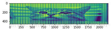
# 将彩色图片降为黑白图片
cat1 = cat.reshape(456,730*3)
plt.imshow(cat1) # 这个办法将图片的形状改变了不好,而且图片看着偏绿色

<matplotlib.image.AxesImage at 0x20f55ef29e8>

# 通过查看cat的数据流可以看出,彩色图片第三维是三个用来表示三原色的数字,那么我们只取其中一个数字,那么原图片
# 就在大小不变的情况下转化为二维黑白图片
# .min  .max  .mean 可以取数组的最大值,最小值,平均值, axis用于确定取值的维度 0 表示第一维
cat2 = cat.min(axis=2) # 取三原色中的小值,图片会偏向黑色
cat3 = cat.max(axis=2) # 取大值,图片偏向白色
cat4 = cat.mean(axis=2) # 取平均值,图片转化为黑白效果最好
plt.imshow(cat3,cmap='gray')
plt.show()
plt.imshow(cat4,cmap='gray')
plt.show()
plt.imshow(cat2,cmap='gray')

<matplotlib.image.AxesImage at 0x20f574c2978>

cat.dtype
# .dtype属性表示数据的类型

dtype('uint8')

cat.astype(np.float64)/255
# .astype 方法可以修改 jpg图片的数据为 0 - 1 的float64类型数据,这样就可以和png格式的图片进行互相交换了

array([[[0.90588235, 0.72941176, 0.51372549],
        [0.90980392, 0.73333333, 0.51764706],
        [0.91372549, 0.7372549 , 0.52156863],
        ...,
        [0.39215686, 0.21176471, 0.21176471],
        [0.36078431, 0.18823529, 0.18431373],
        [0.33333333, 0.16862745, 0.17254902]],

       [[0.90980392, 0.73333333, 0.51764706],
        [0.90980392, 0.73333333, 0.51764706],
        [0.91372549, 0.7372549 , 0.52156863],
        ...,
        [0.39215686, 0.21176471, 0.21176471],
        [0.36078431, 0.18823529, 0.18431373],
        [0.32941176, 0.16470588, 0.16862745]],

       [[0.90980392, 0.73333333, 0.51764706],
        [0.91372549, 0.7372549 , 0.52156863],
        [0.91372549, 0.7372549 , 0.52156863],
        ...,
        [0.38823529, 0.20784314, 0.20784314],
        [0.35686275, 0.18431373, 0.18039216],
        [0.3254902 , 0.16078431, 0.16470588]],

       ...,

       [[0.78039216, 0.46666667, 0.32156863],
        [0.78039216, 0.46666667, 0.32156863],
        [0.78431373, 0.47058824, 0.3254902 ],
        ...,
        [0.74117647, 0.38823529, 0.25490196],
        [0.73333333, 0.38039216, 0.24705882],
        [0.73333333, 0.38039216, 0.24705882]],

       [[0.78039216, 0.46666667, 0.32156863],
        [0.78039216, 0.46666667, 0.32156863],
        [0.78039216, 0.46666667, 0.32156863],
        ...,
        [0.7372549 , 0.38431373, 0.25098039],
        [0.72941176, 0.37647059, 0.24313725],
        [0.7372549 , 0.37254902, 0.24313725]],

       [[0.78039216, 0.46666667, 0.32156863],
        [0.78039216, 0.46666667, 0.32156863],
        [0.78039216, 0.46666667, 0.32156863],
        ...,
        [0.7372549 , 0.38431373, 0.25098039],
        [0.7372549 , 0.37254902, 0.24313725],
        [0.7372549 , 0.37254902, 0.24313725]]])

cat = plt.imread('cat.jpg')
plt.imshow(cat)

<matplotlib.image.AxesImage at 0x20f54379978>

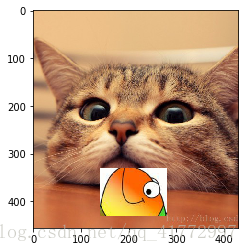
# 下面我们在导入一张鱼的图片它是png格式图片
fish = plt.imread('fish.png')

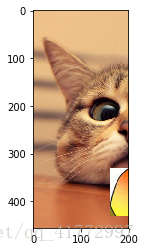
# 假如我们现在要把鱼头放到猫的嘴的位置该怎么做呢?
# 先看鱼和猫图片的大小
fish.shape   # (326,243,3)
cat.shape    # (456,730,3)
# 先把鱼头用切片的办法,切出来
fish_head = fish[50:150,60:200]
# 然后在猫嘴的旁边找到一个 100*140 的区域,然后把鱼头的值赋给它
# 注意,fish是png格式的数据,其值是 0 - 1 的float32类型数据,需要先转换为uint8的数据
fish_head = (fish_head * 255).astype(np.uint8)
# 注意,这里猫图片数据类型有可能是只读类型,需要修改其属性变为可写,不然不可以修改
cat.flags.writeable = True
cat[330:430,260:400] = fish_head
plt.imshow(cat)
# 这样就实现了把鱼头放到猫嘴的操作,同理大家也可以找一下人物肖像进行换头手术
# 这个图片只是完成了简单的效果,如果要进行更加深入的操作,比如鱼头就是圆的,这就需要更加深入的
# 数据分析知识,还有图片颜色看着更加柔和的效果

<matplotlib.image.AxesImage at 0x20f58d80a20>

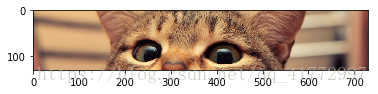
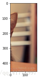
将这张图片切成5张图片呢,或者说本质就是将数据流切成几份

• 按照 y 轴来切

cata = cat[:120]
catb = cat[120:250]
catc = cat[250:]
plt.imshow(cata)
plt.show()
plt.imshow(catb)
plt.show()
plt.imshow(catc)

<matplotlib.image.AxesImage at 0x20f59ecc2b0>

• 按照 x 轴 来切

catax = cat[:, :120]
catbx = cat[:, 120:550]
catcx = cat[:, 550:]
plt.imshow(catax)
plt.show()
plt.imshow(catbx)
plt.show()
plt.imshow(catcx)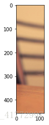

<matplotlib.image.AxesImage at 0x20f58bd0518>

将图片进行上下颠倒,和左右颠倒,以及颜色变换

实质就是改变了数据流的排列方式

• 上下颠倒

cat_top_to_bottom = cat[::-1]
plt.imshow(cat_top_to_bottom)

<matplotlib.image.AxesImage at 0x20f5a9afeb8>

• 左右颠倒

cat_right_to_left = cat[:,::-1]
plt.imshow(cat_right_to_left)
# 注意鱼眼睛跑到左边去了

<matplotlib.image.AxesImage at 0x20f59f24ef0>

• 颜色变换

cat_color_change = cat[:,:,::-1]
plt.imshow(cat_color_change)

<matplotlib.image.AxesImage at 0x20f5a3e9278>

将两张图片拼起来,即将两个数组连接起来

# 为了方便拼接,再导入一张格式和猫一样的dog图片
dog = plt.imread('dog.jpg')
dog.shape # (300, 313, 3) 狗图片比猫图片小,为了拼接需要对锚图片进行裁剪切片
new_cat = cat[100:400,200:513]
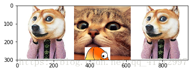
# 使用 numpy.concatenate()函数可以将ndarray的数组级联起来,包括垂直和水平级联
# 此函数的默认参数axis=0,表示垂直级联, axis=1,表示水平级联,也可以说 axis=n表示将第n维数据进行级联
# 并且需要级联的对象要放入到一个元组中作为参数传入,对象在元组中的顺序即级联的顺序
cat_dog_vertical = np.concatenate((dog,new_cat))
cat_dog_horizontal = np.concatenate((dog,new_cat,dog),axis=1)
plt.imshow(cat_dog_vertical)
plt.show()
plt.imshow(cat_dog_horizontal)

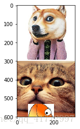
<matplotlib.image.AxesImage at 0x20f5a8e5f60>

通过上面对一张猫的图片的反复操作,我们已经对数据分析,处理有了初步的了解,现在我们系统的对 ndarray | Series | DataFrame几种类型进行深入的了解

首先先看cat的数据类型

type(cat) # numpy.ndarray 类型,这是一种特殊的数组类型,可以有许多的操作

numpy.ndarray

一. numpy.ndarray数组类型

A 生成方式

1. 从Python的数据结构列表,元组等直接转换

nd = np.array([4,5])
nd1 = np.array(([1,2],[3,2],[1,3]))
nd2 = np.array((1,2,3,4,'a','b'))
display(nd,nd1,nd2)

array([4, 5])
array([[1, 2],
       [3, 2],
       [1, 3]])
array(['1', '2', '3', '4', 'a', 'b'], dtype='<U11')

2. 使用np.arange, np.linspace, np.eye, np.logspace, np.eye np.ones, np.zeros, np.full等等八种numpy原生方法

2.1 arange方法: numpy.arange(start, stop, step, dtype=None)它的作用是在给定区间[start,stop)创建一系列均匀间隔的值,这是一个前闭后开的区间,取头不取尾step步长用于设置值的间隔,其值可以是负数.可选参数 dtype可以设置返回的ndarray的类型

nd3 = np.arange(0,150,5)
nd4 = np.arange(100,0,-10)
display(nd3,nd4)

array([  0,   5,  10,  15,  20,  25,  30,  35,  40,  45,  50,  55,  60,
        65,  70,  75,  80,  85,  90,  95, 100, 105, 110, 115, 120, 125,
       130, 135, 140, 145])
array([100,  90,  80,  70,  60,  50,  40,  30,  20,  10])

2.2 linspace方法:numpy.linspace(start, stop, num=50, endpoint=True, retstep=False, dtype=None) 它和arange()差不多都是创建有规律的数组,它可以通过修改参数的方式在指定区间内返回间隔均匀的值

• endpoint:布尔值,如果为真,那么表示可以取到区间的最后一个值
• num: 生成的样本数量. 默认值为50个
• retstep: 布尔值,如果为真,返回间距

nd5 = np.linspace(0,30, num=10, retstep=True, dtype=np.uint8)
nd5

(array([ 0,  3,  6, 10, 13, 16, 20, 23, 26, 30], dtype=uint8),
 3.3333333333333335)

2.3 logspace方法:numpy.logspace(start,stop,num=50,endpoint=True,base=10.0,dtype=None)用于创建规律数组,但是它和linspace有所区别,它有base为底数默认为 10.0

nd6 = np.logspace(0,30,num=10,base=2)
nd6

array([1.00000000e+00, 1.00793684e+01, 1.01593667e+02, 1.02400000e+03,
       1.03212732e+04, 1.04031915e+05, 1.04857600e+06, 1.05689838e+07,
       1.06528681e+08, 1.07374182e+09])

2.4 eye方法:numpy.eye(N,M,k=0,dtype=None) 用于创建一个二维数组,特定k对角线上的值为1,其余值全部为0

• N: 输出数组行数
• M: 输出数组列数
• k: 对角线索引,默认为 0,指主对角线,正值指上对角线,赋值指下对角线

nd7 = np.eye(3,3)
nd8 = np.eye(3,3,k=1)
nd9 = np.eye(3,3,k=-1)
display(nd7,nd8,nd9)

array([[1., 0., 0.],
       [0., 1., 0.],
       [0., 0., 1.]])
array([[0., 1., 0.],
       [0., 0., 1.],
       [0., 0., 0.]])
array([[0., 0., 0.],
       [1., 0., 0.],
       [0., 1., 0.]])

2.5 diag方法: np.diag(v,k=0)用于构建对角矩阵(这是一个满秩矩阵)

• v: 一维或者二维数组
• k: k < 0 表示斜线在矩阵下方, k > 0 表示斜线在矩阵上方

nd10 = np.diag([1,2,3])
nd10

array([[1, 0, 0],
       [0, 2, 0],
       [0, 0, 3]])

2.6 ones方法:numpy.ones(shape,dtype=None,order='C')用于快速创建数值全部为1的多维数组

• shape: 用于指定数组的形状维度
• order: {'C','F'}, 表示按行或者列方式存储数组

nd5 = np.ones(shape=(2,3,4))
nd5

array([[[1., 1., 1., 1.],
        [1., 1., 1., 1.],
        [1., 1., 1., 1.]],    
       [[1., 1., 1., 1.],
        [1., 1., 1., 1.],
        [1., 1., 1., 1.]]])

2.7 zeros方法:`numpy.zeros(shape,dtype=None,order=’C’),它与ones方法非常相似,只是全部数值为 0 的区别

nd6 = np.zeros(shape=(2,3,4))
nd6 

array([[[0., 0., 0., 0.],
        [0., 0., 0., 0.],
        [0., 0., 0., 0.]],

       [[0., 0., 0., 0.],
        [0., 0., 0., 0.],
        [0., 0., 0., 0.]]])

2.8 full方法:numpy.full(shape,fill_value=num)用于创建一个自定义形状的数组,可以自己指定一个值,用它填满整个数组

• fill_value: 用来填充的值,可以是数字,也可以是字符串

nd7 = np.full(shape=(2,3,4),fill_value='ai')
nd7

array([[['ai', 'ai', 'ai', 'ai'],
        ['ai', 'ai', 'ai', 'ai'],
        ['ai', 'ai', 'ai', 'ai']],

       [['ai', 'ai', 'ai', 'ai'],
        ['ai', 'ai', 'ai', 'ai'],
        ['ai', 'ai', 'ai', 'ai']]], dtype='<U2')

3. 文件 I/O 创建数组

csv, dat 是常见的数据格式化文件类型,从中读取数据可以使用numpy.genfromtxt()

首先我们先生成一个.dat的文件
使用 numpy.savetxt 我们可以将 Numpy 数组保存到csv文件中
不管给什么样的后缀名，都会以txt的格式进行存储

M = np.full(shape=(3,3),fill_value=11,dtype=np.uint8)
np.savetxt("random-matrix.dat", M)

#函数。
data1=np.genfromtxt('./random-matrix.dat')
print(data1.shape) #(3.3)

data2=np.loadtxt('./random-matrix.dat')
print(data2.shape)  #(3.3)

data3=np.mafromtxt('./random-matrix.dat')
print(data3.shape)  #(3.3)

data4=np.ndfromtxt('./random-matrix.dat')
print(data4.shape) #(3.3)

data5=np.recfromtxt('./random-matrix.dat')
print(data5.shape) #(3.3)

可以使用 numpy.save 和 numpy.load 进行保存和读取:

# 保存和读取的文件格式为 .npy
M1 = np.save('newfile.npy',M)
M2 = np.load('newfile.npy')
M2

array([[11, 11, 11],
       [11, 11, 11],
       [11, 11, 11]], dtype=uint8)

4. 使用特殊函数创建数组,比如random

• 生成随机的整数矩阵
  numpy.random.randint(low,high=None,size,dtype='1')
  
  • low: 最小值,可以取到
  • high: 最大值,不可取到
  • size: 数组形状维度,是个元组值
  • dtype: 数据类型,默认’1’

np.random.randint(0,10,size=(5,4))

array([[7, 6, 9, 1],
       [5, 8, 6, 6],
       [2, 2, 6, 5],
       [1, 9, 5, 1],
       [3, 6, 6, 0]])

• 生成符合标准正太分布的矩阵np.random.randn(d0,d1...dn)
  
  • dn: 每多一个参数表示增加一个维度,数组总长度等于,d1 * d2 * … * dn

np.random.randn(3,5)

array([[ 0.8512631 , -0.89151525,  0.17230815,  1.226017  ,  0.15265477],
       [ 0.83407878, -0.20524797,  0.90489634,  2.10492139, -1.34583095],
       [-1.21030368, -1.53301206, -0.53699127, -0.75694624,  0.78337365]])

• 生成 0 -1 的小数的随机矩阵np.random.random(size=None)
  
  • size: 表示数组的形状与维度

np.random.random(size=(3,2))

array([[0.63842185, 0.95487669],
       [0.6678316 , 0.3371709 ],
       [0.11624348, 0.00438239]])

• 生成一个符合指定要求的正太分布的一维数组np.random.normal(loc=0.0,scale=1.0,size=None)
<ul><li>loc: location是定位的值</li>
<li>scale: 数据的波动值</li>
<li>size: 数据的长度</li>
<li>normal` 也是一个正太分布的方法

# 生成一个定位值 5,波动值 2 ,长度 20 的一维数组
np.random.normal(loc=5,scale=2,size=20)

array([6.62285072, 2.52593   , 4.74308815, 3.12310272, 5.93661179,
       5.35622566, 5.9867008 , 3.43611194, 3.11771284, 2.73816327,
       1.53143852, 4.12338866, 7.83855536, 8.85641589, 5.52196218,
       6.21622332, 7.48189175, 4.26170198, 7.41470467, 3.30858065])

• 生成一个随机数的矩阵np.random.rand(d0,d1...dn)用来生成一个随机数的多维矩阵

np.random.rand(2,3,4)

array([[[0.07317866, 0.10858634, 0.31782862, 0.50225594],
        [0.15306118, 0.80909035, 0.15104803, 0.34185875],
        [0.11788373, 0.22802125, 0.8065444 , 0.80557928]],

       [[0.04196403, 0.3676074 , 0.34386995, 0.09118787],
        [0.68947718, 0.59828665, 0.47979887, 0.74415499],
        [0.08056806, 0.51031884, 0.15978529, 0.76386364]]])

B ndarray 数组属性

• ndim: 数组的维度
• shape: 数组形状 (5,4,3)
• size: 数组的总长度
• dtype: 查看数据类型

1. ndarray.T

ndarray.T 用于二维数组转置,与np.transpose()效果相同

# 首先生成一个二维矩阵
nd = np.random.randint(0, 10, size=(3,4))
nd

array([[0, 3, 3, 0],
       [7, 5, 7, 3],
       [3, 8, 8, 6]])

nd.T

array([[0, 7, 3],
       [3, 5, 8],
       [3, 7, 8],
       [0, 3, 6]])

nd.transpose()
np.transpose(nd)
# 两种写法都可以

array([[0, 7, 3],
       [3, 5, 8],
       [3, 7, 8],
       [0, 3, 6]])

2. ndarray.imag 输出数组所有元素的虚部,没有虚部则为0

nd.imag
np.imag(nd)
# 两种写法

array([[0, 0, 0, 0],
       [0, 0, 0, 0],
       [0, 0, 0, 0]])

3. ndarray.real输出数组所有元素的实部

nd.real
np.real(nd)
# 两种写法都可以

array([[0, 3, 3, 0],
       [7, 5, 7, 3],
       [3, 8, 8, 6]])

4. ndarray.itemsize输出数组元素的字节数

nd.dtype 
# int8类型的数据 占1个字节
# int32类型的数据 占4个字节
# int64类型的数据 占8个字节
nd.itemsize

4

5. ndarray.nbytes输出数组元素总字节数

nd # 已知数组

array([[0, 3, 3, 0],
       [7, 5, 7, 3],
       [3, 8, 8, 6]])

nd.dtype

dtype('int32')

nd.nbytes
# nd是3 * 4 的二维数组,它的元素是int32类型占4个字节,一共12个元素,所以总字节为12*4=48

48

6. ndarray.strides输出遍历数组是每个维度中数组的总字节数

nd.strides
# nd 是 3*4 的二维数组,元素是int32类型
# 第一维有3个对象,每个对象是一个数组,数组中有4个基本元素,因此每个对象的总字节数为 4 * 4 = 16
# 第二维有4个基本元素,每个元素4个字节

(16, 4)

C 对Numpy数组的基本操作

在前面对猫的图片进行,换鱼头,颠倒,切片就是一些基本的操作,下面介绍一些新的操作

1. ravel()方法: 将任意数组扁平化,即将任意数组变为一维数组

nd.ravel() # 变成一位数组

array([0, 3, 3, 0, 7, 5, 7, 3, 3, 8, 8, 6])

2. concatenate()方法: np.concatenate((a0,a1...an), axis=0,out=None)

• 级联参数是列表,一定要加()或者[]
• 参加级联的数组维度必须相同
• 形状相同,axis表示级联时的方向,默认 axis=0 从第一维开始级联,那么每个数组在这一维度的数量必须相同
• 对于两个二维数组a,b: 水平级联时a,b的行数必须相同,列数随意;垂直级联时列数必须相同,行数随意

nd1 = np.random.randint(0,10,size=(3,4))
nd2 = np.random.randint(0,10,size=(3,4))
nd3 = np.random.randint(0,10,size=(3,2))
nd4 = np.random.randint(0,10,size=(4,4))
# nd1 和 nd2 可以进行任意级联
a = np.concatenate((nd1,nd2),axis=1)
b = np.concatenate((nd1,nd2),axis=0)
# nd1 和 nd3 可以进行水平级联
c = np.concatenate((nd1,nd3),axis=1)
# nd1 和 nd4 可以进行垂直级联
d = np.concatenate((nd1,nd4),axis=0)
# nd3 和 nd4 不能进行级联

display(a,b,c,d)

array([[9, 4, 8, 3, 5, 2, 9, 0],
       [5, 2, 5, 4, 0, 4, 9, 2],
       [6, 6, 4, 3, 3, 1, 8, 6]])
array([[9, 4, 8, 3],
       [5, 2, 5, 4],
       [6, 6, 4, 3],
       [5, 2, 9, 0],
       [0, 4, 9, 2],
       [3, 1, 8, 6]])
array([[9, 4, 8, 3, 1, 5],
       [5, 2, 5, 4, 5, 2],
       [6, 6, 4, 3, 9, 8]])
array([[9, 4, 8, 3],
       [5, 2, 5, 4],
       [6, 6, 4, 3],
       [6, 7, 6, 5],
       [4, 6, 3, 2],
       [4, 7, 7, 4],
       [8, 1, 7, 2]])

3. numpy.[hstack | vstack] 一种特殊的级联方式

.hstack 表示水平级联
.vstack 表示垂直级联

nd_h = np.hstack((nd1,nd2))
nd_v = np.vstack((nd1,nd2))
display(nd_h, nd_v)

array([[9, 4, 8, 3, 5, 2, 9, 0],
       [5, 2, 5, 4, 0, 4, 9, 2],
       [6, 6, 4, 3, 3, 1, 8, 6]])
array([[9, 4, 8, 3],
       [5, 2, 5, 4],
       [6, 6, 4, 3],
       [5, 2, 9, 0],
       [0, 4, 9, 2],
       [3, 1, 8, 6]])

4. 分割数组

在前面处理猫图片的时候已经进行过切片分割,这里采用np.split(ary, indices_or_sections, axis=0)函数方法
- ary: 需要分割的数组
- indices_or_sections: 需要将数组切成几份,切出来的大小
- axis: 按照那个维度进行分割,默认为 0,从y轴切割

这里还是使用猫的图片进行分割

plt.imshow(cat)
# 把猫沿y轴进行分割为3份
cat1,cat2,cat3 = np.split(cat,[100,300])
plt.imshow(cat1)
plt.show()
plt.imshow(cat2)
plt.show()
plt.imshow(cat3)

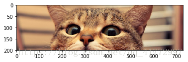
<matplotlib.image.AxesImage at 0x20f5afd9828>

plt.imshow(cat)
# 把猫沿x轴进行分割为3份
cat1,cat2,cat3 = np.split(cat,[100,300],axis=1)
plt.imshow(cat1)
plt.show()
plt.imshow(cat2)
plt.show()
plt.imshow(cat3)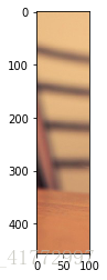

<matplotlib.image.AxesImage at 0x20f5a7806a0>

5. 副本

所有赋值运算都不会为ndarray的任何元素创建副本.对赋值后对象的操作对原来的对象也是生效的
可以使用ndarray.copy()函数创建副本 — 即深拷贝

cat_new = cat.copy()
display(id(cat_new),id(cat))

2264965411584
2264860738384

6. ndarray的聚合函数

• 求和np.sum(axis=None, dtype=None, out=None, keepdims=False)
  
  • axis:表示求和的维度,不写表示对所有元素进行求和,对于多维数组,axis的值可以是一个元组,可以表示对多个维度进行求和

nd

array([[0, 3, 3, 0],
       [7, 5, 7, 3],
       [3, 8, 8, 6]])

nd.sum() # nd中所有元素的和 53
nd.sum(axis=1) # nd中第二维元素的和 array([ 6, 22, 25])
nd.sum(axis=0) # nd中第一维元素的和 array([10, 16, 18,  9])

• 最大最小平均值: np.max / np.min / np.mean 它们都有一个axis关键字参数,可以确定是求哪一个维度的值,如果不写,表示求所有元素和的对应值

nd

array([[0, 3, 3, 0],
       [7, 5, 7, 3],
       [3, 8, 8, 6]])

a = nd.min(axis=1) # 最小值array([0, 3, 3])
b = nd.max(axis=1) # 最大值array([3, 7, 8])
c = nd.mean(axis=0) # 平均值array([3.33333333, 5.33333333, 6.        , 3.        ])

• 其它一些聚合操作

Function Name	NaN-safe Version	Description
np.sum	np.nansum	Compute sum of elements
np.prod	np.nanprod	Compute product of elements
np.mean	np.nanmean	Compute mean of elements
np.std	np.nanstd	Compute standard deviation
np.var	np.nanvar	Compute variance
np.min	np.nanmin	Find minimum value
np.max	np.nanmax	Find maximum value
np.argmin	np.nanargmin	Find index of minimum value 找到最小数的下标
np.argmax	np.nanargmax	Find index of maximum value
np.median	np.nanmedian	Compute median of elements
np.percentile	np.nanpercentile	Compute rank-based statistics of elements
np.any	N/A	Evaluate whether any elements are true
np.all	N/A	Evaluate whether all elements are true
np.power	N/A	幂运算
np.argwhere(nd1<0)	N/A	N/A

7. 轴移动

• moveaxis()方法: numpy.moveaxis(a,source,destination) 可以将数组的轴移动到指定的位置
  
  • a: 数组
  • source: 要移动的轴的原始位置
  • destination: 要移动轴的目标位置

# 创建一个特殊数组,便于演示
nd = np.array([[1,2,3],[1,2,3],[1,2,3]])
# 将nd的 x 轴 与 y 轴进行互换
np.moveaxis(nd,0,1)

array([[1, 1, 1],
       [2, 2, 2],
       [3, 3, 3]])

8. 轴交换

*swapaxes()方法:np.swapsxes(a,axis1,axis2) 与moveaxis不同,swapaxes可以交换数组的任意轴,任意维度之间进行交换
- a: 数组
- axis1: 需要交换的轴1(维度a)的位置
- axis2: 需要与轴1(维度a)进行交换的轴2(维度b)的位置

# 创建一个 多维数组
ndx = np.random.randint(0,100,size=(3,4,5))
# 将第一维与第三维进行交换
ndx1 = np.swapaxes(ndx, 0,2)
display(ndx,ndx1)

array([[[93, 81, 22, 66, 14],
        [69, 12, 48, 84, 76],
        [96, 59, 25, 49, 21],
        [57, 83, 32, 51, 29]],

       [[52, 47, 29, 58, 18],
        [79, 34, 11, 75, 40],
        [11, 31, 43, 84, 73],
        [60, 88, 33, 46, 51]],

       [[93, 95, 76, 59, 76],
        [20, 20, 21, 10, 85],
        [ 3, 20, 97, 26, 25],
        [79, 53, 60, 85, 88]]])

array([[[93, 52, 93],
        [69, 79, 20],
        [96, 11,  3],
        [57, 60, 79]],

       [[81, 47, 95],
        [12, 34, 20],
        [59, 31, 20],
        [83, 88, 53]],

       [[22, 29, 76],
        [48, 11, 21],
        [25, 43, 97],
        [32, 33, 60]],

       [[66, 58, 59],
        [84, 75, 10],
        [49, 84, 26],
        [51, 46, 85]],

       [[14, 18, 76],
        [76, 40, 85],
        [21, 73, 25],
        [29, 51, 88]]])