
在前一篇文章中,我们介绍了如何使用 Amazon EC2 Inf2 实例部署大语言模型,有不少用户询问 Amazon Inf2 实例是否支持当下流行的 AIGC 模型,答案是肯定的。同时,图片生成时间、QPS、服务器推理成本、如何在云中部署,也是用户关心的话题。
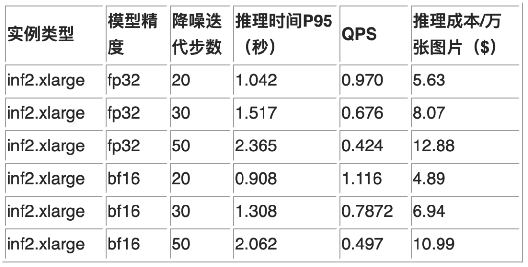
首先我们看一下 HuggingFace Stable Diffusion 2.1(512×512)在 inferentia2 上的表现。实验使用了 Amazon EC2 inf2.xlarge 实例,采样器使用 DPMSolverMultistepScheduler,模型的精度对比了 fp32 和 bfloat16,降噪步数选择了 20,30 和 50 步,inf2 的价格参照美东二区(Ohio)的按需实例价格。从结果中我们可以看出,在降噪迭代步数为 20 时,生成图片的时间在 1 秒左右。
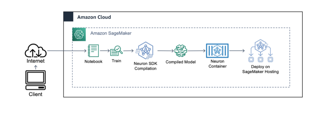
在本篇文章中,我们将介绍如何在 Amazon SageMaker 环境中使用 Inf2 实例部署 Stable Diffusion V2.1 模型。下面我们简要介绍一下将模型 Stable Diffusion 2.1 部署到 Amazon SageMaker 的过程中用到的几个工具。
Neuron SDK
Amazon Neuron 是用于在基于 Amazon Inferentia 和 Amazon Trainium 的实例上运行深度学习工作负载的开发工具包。它支持客户在其端到端 ML 开发生命周期中构建新模型、训练和优化这些模型,然后将它们部署到生产环境中。
模型包括编译和运行两个阶段,对于编译阶段,可以在 inf2 实例上进行,同样可以在 m、r、c 系列的 EC2 实例上进行;对于运行阶段,需要在 inf2 实例上运行。
在最近发布的 Neuron SDK 2.10 中,增加了对 Stable Diffusion 模型的支持,详细信息请参考 Neuron SDK 2.10。
Stable Diffusion 模型
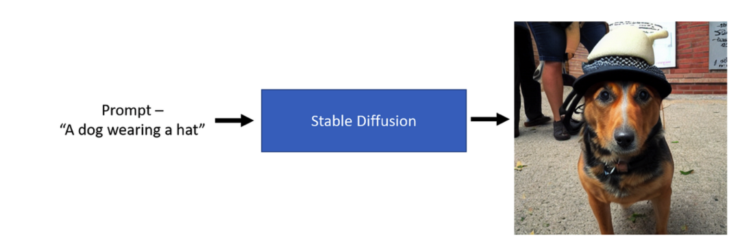
Stable Diffusion 是一个文本到图像的潜在扩散模型(Latent Diffusion Model),由 CompVis、Stability AI 和 LAION 的研究人员和工程师创建。它使用来自 LAION-5B 数据库子集的 512×512 图像进行训练。
扩散模型是一种生成模型,用于生成与训练数据相似的数据。简单的说,扩散模型的工作方式是通过迭代添加高斯噪声来“破坏”训练数据,然后学习如何消除噪声来恢复数据。
Stable Diffusion 模型各部分功能如下:
VAE Encoder:负责对输入图像进行压缩。
VAE Decoder:负责对潜空间输出结果进行放大(超分辨率)。
Clip Text Encoder:负责对输入的提示(Prompt)进行编码,即把文本信息转换为向量的表示。
Unet:负责进行反向扩散过程中的噪声预测。
从 Stable Diffusion 的功能不难看出,模型包含了 3 个子模型 Clip,VAE 和 UNet。在后面的介绍中,我们会对三个模型在 Amazon Inf2 上进行编译。
Amazon Inferentia2 支持的数据类型
Inferentia2 支持 FP32、TF32、BF16、FP16、UINT8 和新的可配置 FP8 (cFP8) 数据类型。Amazon Neuron 可以采用高精度 FP32 和 FP16 模型并将它们自动转换为精度较低的数据类型,同时优化准确性和性能。Autocasting 通过消除对低精度再训练的需求并使用更小的数据类型实现更高性能的推理。
FP32 是单精度浮点数,占用 4 个字节,共 32 位。前 8bit 表示指数,后 23bit 表示小数;FP16 半精度浮点数,占用 2 个字节,共 16 位,前 5bit 表示指数,后 10bit 表示小数;BF16 是对 FP32 单精度浮点数截断数据,即用 8bit 表示指数,7bit 表示小数。
在数据表示范围上,FP32 和 BF16 表示的整数范围是一样的,小数部分表示不一样,存在舍入误差;FP32 和 FP16 表示的数据范围不一样,在计算中,FP16 存在溢出风险;BF16 和 FP16 在精度上不一样,BF16 可表示的整数范围更广泛,但是尾数精度较小;FP16 表示整数范围较小,但是尾数精度较高。
与 FP32 位相比,采用 BF16/FP16 吞吐量可以翻倍,内存需求可以减半。因此在一些推理场景中,在精度满足要求的前提下,会把模型转换为 BF16/FP16 格式。
为了使读者能更充分了解 BF16,在下文的实验中,我们将采用 BF16 供大家学习参考。
DJL- Serving
上文中我们提到了部署,那么就需要一个 web 容器去部署模型。DJLServing 是与编程语言无关的 DJL(Deep Java Library)提供支持的高性能通用模型服务解决方案。它可以服务于常见的模型类型,例如 PyTorch TorchScript、TensorFlow SavedModel、ONNX、TensorRT 模型。
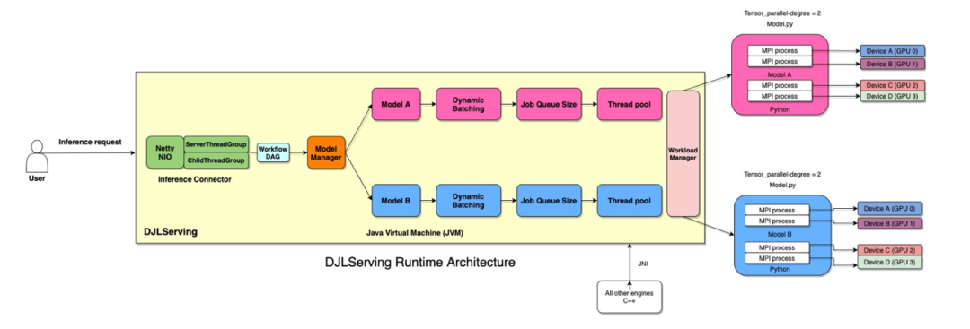
DJLServing 是用多层组成,路由层建立在 Netty 之上。远程请求在路由层中处理,分发给工作线程 Worker(Java 中的线程或 Python 中的进程)运行推理。机器的 Java 线程总数设置为 2 * cpu_core,以充分利用计算能力。Worker 数量可以根据型号或 DJL 在硬件上的自动检测进行配置。下图说明了 DJLServing 的架构。
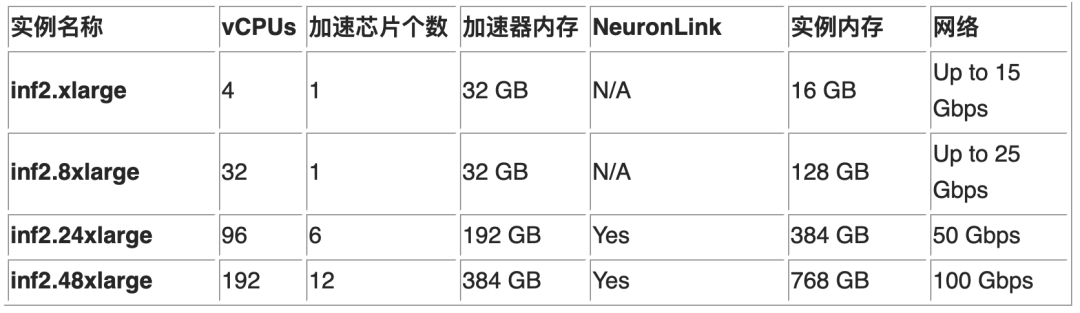
Amazon Inf2 实例类型
下表详细列出了 Inf2 EC2 实例的大小和规格。对于 Stable Diffusion 的模型,我们可以部署在下面的任何一种类型的实例上。在 SageMaker 中,Inf2 的实例规格与 EC2 实例完全相同,SageMaker 中的 Inf2 实例加上了前缀 ml,比如 inf2.xlarge 在 SageMaker 中对应 ml.inf2.xlarge。
实验步骤
进入 Amazon 控制台,切换到 us-east-2 区域,然后导航到 SageMaker 控制台,启动一台 ml.m5.2xlarge Notebook 实例或者同等内存的实例类型,EBS 存储选择 50G,新建一个 Role 具有 AmazonSageMakerFullAccess 和 AmazonS3FullAccess 两个 policy,并把新创建的 Role 附加到 Notebook 实例上。
在 Notebook 启动后,进入 terminal 下载 Notebook 脚本。
wget https://d1m6v8zdux9m8v.cloudfront.net/SageMaker_INF2_SD21_inference.ipynb左滑查看更多
打开 SageMaker_INF2_SD21_inference.ipynb,Kernel 选择conda_pytorch_p310。实验步骤主要分为如下几步:
1. 实验前的准备
由于部署用到 inf2 实例,SageMaker Hosting 有至少一个 inf2 配额。Stable Diffusion 可以部署在 ml.inf2.xlarge,ml.inf2.8xlarge,ml.inf2.48xlarge 或者 ml.inf2.24xlarge 实例上。
2. 环境配置
我们会在 Notebook 实例上编译模型,因此需要安装编译模型需要的 Neuron-cc 和常用的软件包。
3. 模型编译
在我们创建的 ml.m5.2xlarge 笔记本实例上编译 Stable Diffusion2.1 模型。
4. 准备部署脚本
我们采用 BYOS(Bring Your Own Script)的方式,准备脚本文件并打包上传到 S3。脚本文件主要负责模型的加载以及处理推理请求。
5. 准备模型文件
准备待部署的模型文件并上传到 S3。
6. 模型部署
在 SageMaker 中部署模型。
7. 测试验证
依次执行单元格内容,并观察每一步的执行结果。
下面我们解释编译的主要代码内容:
以下代码块定义了一个用于 UNet 的双重包装器和一个用于文本编码器的另一个包装器。这些包装器使得 torch_neuronx.trace 能够追踪被包装的模型以便使用 Neuron 编译器进行编译。此外,get_attention_scores 实用函数执行了优化的注意力分数计算,并通过补丁(参见下一个代码块中的”Compile UNet and save”部分的用法)替换 diffusers 包中原始的 get_attention_scores 函数。
class UNetWrap(nn.Module):
    def __init__(self, unet):
        super().__init__()
        self.unet = unet


    def forward(self, sample, timestep, encoder_hidden_states, cross_attention_kwargs=None):
        out_tuple = self.unet(sample, timestep, encoder_hidden_states, return_dict=False)
        return out_tuple


class NeuronUNet(nn.Module):
    def __init__(self, unetwrap):
        super().__init__()
        self.unetwrap = unetwrap
        self.config = unetwrap.unet.config
        self.in_channels = unetwrap.unet.in_channels
        self.device = unetwrap.unet.device


    def forward(self, sample, timestep, encoder_hidden_states, cross_attention_kwargs=None):
        sample = self.unetwrap(sample, timestep.float().expand((sample.shape[0],)).to(torch.bfloat16), encoder_hidden_states)[0]
        return UNet2DConditionOutput(sample=sample)


class NeuronTextEncoder(nn.Module):
    def __init__(self, text_encoder):
        super().__init__()
        self.neuron_text_encoder = text_encoder
        self.config = text_encoder.config
        self.dtype = text_encoder.dtype
        self.device = text_encoder.device


    def forward(self, emb, attention_mask = None):
        return [self.neuron_text_encoder(emb)['last_hidden_state']]


# Optimized attention
def get_attention_scores(self, query, key, attn_mask):
    dtype = query.dtype


    if self.upcast_attention:
        query = query.float()
        key = key.float()


    # Check for square matmuls
    if(query.size() == key.size()):
        attention_scores = custom_badbmm(
            key,
            query.transpose(-1, -2)
        )


        if self.upcast_softmax:
            attention_scores = attention_scores.float()


        attention_probs = torch.nn.functional.softmax(attention_scores, dim=1).permute(0,2,1)
        attention_probs = attention_probs.to(dtype)


    else:
        attention_scores = custom_badbmm(
            query,
            key.transpose(-1, -2)
        )


        if self.upcast_softmax:
            attention_scores = attention_scores.float()


        attention_probs = torch.nn.functional.softmax(attention_scores, dim=-1)
        attention_probs = attention_probs.to(dtype)

    return attention_probs


def custom_badbmm(a, b):
    bmm = torch.bmm(a, b)
    scaled = bmm * 0.125
    return scaled
左滑查看更多
下列代码是模型编译的主要部分。首先定义了模型的 id 以及编译结果输出的路径,然后依次对 Clip text_encoder、UNET 和 VAE 三个模型进行编译。这里读者应注意到数据格式采用 torch.bfloat16。在这个过程中,会使用到大量内存。我们通过调用 del 函数清理不使用的内存。
# For saving compiler artifacts
COMPILER_WORKDIR_ROOT = 'sd2_compile_dir_512'
# Model ID for SD version pipeline
model_id = "stabilityai/stable-diffusion-2-1-base"


# --- Compile CLIP text encoder and save ---
# Only keep the model being compiled in RAM to minimze memory pressure
pipe = StableDiffusionPipeline.from_pretrained(model_id, torch_dtype=torch.bfloat16)
pipe.save_pretrained(COMPILER_WORKDIR_ROOT) # save original model
text_encoder = copy.deepcopy(pipe.text_encoder)
del pipe
# Apply the wrapper to deal with custom return type
text_encoder = NeuronTextEncoder(text_encoder)
# Compile text encoder
# This is used for indexing a lookup table in torch.nn.Embedding,
# so using random numbers may give errors (out of range).
emb = torch.tensor([[49406, 18376,   525,  7496, 49407,     0,     0,     0,     0,     0,
        0,     0,     0,     0,     0,     0,     0,     0,     0,     0,
        0,     0,     0,     0,     0,     0,     0,     0,     0,     0,
        0,     0,     0,     0,     0,     0,     0,     0,     0,     0,
        0,     0,     0,     0,     0,     0,     0,     0,     0,     0,
        0,     0,     0,     0,     0,     0,     0,     0,     0,     0,
        0,     0,     0,     0,     0,     0,     0,     0,     0,     0,
        0,     0,     0,     0,     0,     0,     0]])
text_encoder_neuron = torch_neuronx.trace(
        text_encoder.neuron_text_encoder,
        emb,
        compiler_workdir=os.path.join(COMPILER_WORKDIR_ROOT, 'text_encoder'),
        )
# Save the compiled text encoder
text_encoder_filename = os.path.join(COMPILER_WORKDIR_ROOT, 'text_encoder/model.pt')
torch.jit.save(text_encoder_neuron, text_encoder_filename)
# delete unused objects
del text_encoder
del text_encoder_neuron


# --- Compile VAE decoder and save ---
# Only keep the model being compiled in RAM to minimze memory pressure
pipe = StableDiffusionPipeline.from_pretrained(model_id, torch_dtype=torch.bfloat16)
decoder = copy.deepcopy(pipe.vae.decoder)
del pipe
# Compile vae decoder
decoder_in = torch.randn([1, 4, 64, 64]).to(torch.bfloat16)
decoder_neuron = torch_neuronx.trace(
    decoder,
    decoder_in,
    compiler_workdir=os.path.join(COMPILER_WORKDIR_ROOT, 'vae_decoder'),
)
# Save the compiled vae decoder
decoder_filename = os.path.join(COMPILER_WORKDIR_ROOT, 'vae_decoder/model.pt')
torch.jit.save(decoder_neuron, decoder_filename)
# delete unused objects
del decoder
del decoder_neuron


# --- Compile UNet and save ---
pipe = StableDiffusionPipeline.from_pretrained(model_id, torch_dtype=torch.bfloat16)
# Replace original cross-attention module with custom cross-attention module for better performance
CrossAttention.get_attention_scores = get_attention_scores
# Apply double wrapper to deal with custom return type
pipe.unet = NeuronUNet(UNetWrap(pipe.unet))
# Only keep the model being compiled in RAM to minimze memory pressure
unet = copy.deepcopy(pipe.unet.unetwrap)
del pipe
# Compile unet
sample_1b = torch.randn([1, 4, 64, 64]).to(torch.bfloat16)
timestep_1b = torch.tensor(999).float().expand((1,)).to(torch.bfloat16)
encoder_hidden_states_1b = torch.randn([1, 77, 1024]).to(torch.bfloat16)
example_inputs = sample_1b, timestep_1b, encoder_hidden_states_1b
unet_neuron = torch_neuronx.trace(
    unet,
    example_inputs,
    compiler_workdir=os.path.join(COMPILER_WORKDIR_ROOT, 'unet'),
    compiler_args=["--model-type=unet-inference"]
)
# save compiled unet
unet_filename = os.path.join(COMPILER_WORKDIR_ROOT, 'unet/model.pt')
torch.jit.save(unet_neuron, unet_filename)
# delete unused objects
del unet
del unet_neuron


# --- Compile VAE post_quant_conv and save ---
# Only keep the model being compiled in RAM to minimze memory pressure
pipe = StableDiffusionPipeline.from_pretrained(model_id, torch_dtype=torch.bfloat16)
post_quant_conv = copy.deepcopy(pipe.vae.post_quant_conv)
del pipe
# # Compile vae post_quant_conv
post_quant_conv_in = torch.randn([1, 4, 64, 64]).to(torch.bfloat16)
post_quant_conv_neuron = torch_neuronx.trace(
    post_quant_conv,
    post_quant_conv_in,
    compiler_workdir=os.path.join(COMPILER_WORKDIR_ROOT, 'vae_post_quant_conv'),
)
# # Save the compiled vae post_quant_conv
post_quant_conv_filename = os.path.join(COMPILER_WORKDIR_ROOT, 'vae_post_quant_conv/model.pt')
torch.jit.save(post_quant_conv_neuron, post_quant_conv_filename)
# delete unused objects
del post_quant_conv
del post_quant_conv_neuron
左滑查看更多
运行完成后,编译结果保存在 sd2_compile_dir_512 文件夹下,同时原始 Stable Diffusion2.1 模型保存在 sd2_512_root。在模型加载中,我们会把原始模型和编译后的模型放在目录 sd2_512_root。
%%bash
mkdir sd2_512_root/compiled_models #创建文件路径
cp sd2_compile_dir_512/text_encoder/model.pt sd2_512_root/compiled_models/text_encoder.pt
cp sd2_compile_dir_512/unet/model.pt sd2_512_root/compiled_models/unet.pt
cp sd2_compile_dir_512/vae_decoder/model.pt sd2_512_root/compiled_models/vae_decoder.pt
cp sd2_compile_dir_512/vae_post_quant_conv/model.pt sd2_512_root/compiled_models/vae_post_quant_conv.pt
sd2_512_root文件层级如下所示:
(aws_neuron_venv_pytorch) sh-4.2$ tree
.
├── compiled_models
│   ├── text_encoder.pt
│   ├── unet.pt
│   ├── vae_decoder.pt
│   └── vae_post_quant_conv.pt
├── feature_extractor
│   └── preprocessor_config.json
├── model_index.json
├── scheduler
│   └── scheduler_config.json
├── text_encoder
│   ├── config.json
│   └── pytorch_model.bin
├── tokenizer
│   ├── merges.txt
│   ├── special_tokens_map.json
│   ├── tokenizer_config.json
│   └── vocab.json
├── unet
│   ├── config.json
│   └── diffusion_pytorch_model.bin
└── vae
    ├── config.json
    └── diffusion_pytorch_model.bin
左滑查看更多
准备部署脚本
我们采用 BYOS(Bring Your Own Script)的方式,在文件 model.py 中,定义了 load_model,run_inference 和 handle 方法,容器启动后会加载 model.py 并执行。
部署脚本中还包含了 serving.properties,里面定义了部署 DJL- Serving 用到的参数。
engine – 指定将用于此工作负载的引擎。在这种情况下,我们将使用 DJL Python Engine 来托管模型。
option.entryPoint – 指定用于托管模型的入口代码。djl_python.huggingface 是来自 djl_python 仓库的 huggingface.py 模块。
option.s3url – 指定模型文件的位置。或者可以使用 option.model_id 选项来指定来自 Hugging Face Hub 的模型(例如 EleutherAI/gpt-j-6B),模型将自动从 Hub 下载。推荐使用 s3url 方法,因为它允许您在自己的环境中托管模型文件,并通过 DJL 推理容器内的优化方法从 S3 将模型传输到托管实例,从而实现更快的部署。
option.task – 这是针对 huggingface.py 推理处理程序的特定选项,用于指定将用于哪个任务的模型。
option.tensor_parallel_degree – 通过分层模型划分实现模型的张量并行化。
option.load_in_8bit – 将模型权重量化为 int8,从而大大减小模型在内存中的占用空间,从初始的 FP32 减少。
下面的脚本打包自定义的脚本并上传到 S3。
boto3_s3_client = boto3.client("s3",region_name='us-east-2',**boto3_kwargs)
boto3_s3_client.upload_file("./model.tar.gz", bucket, f"{s3_code_prefix}/model.tar.gz") # - "path/to/key.txt"


s3_code_artifact = f"s3://{bucket}/{s3_code_prefix}/model.tar.gz"
print(f"S3 Code or Model tar ball uploaded to --- > {s3_code_artifact}")
boto3_s3_client.list_objects(Bucket=bucket, Prefix=f"{s3_code_prefix}/model.tar.gz").get('Contents', [])
print(f"S3 Model Prefix where the model files are -- > {s3_model_prefix}")
print(f"S3 Model Bucket is -- > {bucket}")
左滑查看更多
上传 model.tar.gz 到 s3://<s3_bucket>/stablediffusion/neuron/code_sd/model.tar.gz 路径下。
SageMaker 部署推理节点
在 us-east-2,stable diffusion inf2 对应 ECR 镜像 URI 为:
inference_image_uri = "763104351884.dkr.ecr.us-east-2.amazonaws.com/djl-inference:0.22.1-neuronx-sdk2.10.0"左滑查看更多
之后使用 SageMaker 客户端创建一个具有指定名称、执行角色和主要容器的模型,并将打印出模型的 ARN。
from sagemaker.utils import name_from_base
boto3_sm_client = boto3.client("sagemaker",region_name='us-east-2',**boto3_kwargs)
model_name = name_from_base(f"inf2-sd")
create_model_response = boto3_sm_client.create_model(
    ModelName=model_name,
    ExecutionRoleArn=role,
    PrimaryContainer={"Image": inference_image_uri, "ModelDataUrl": s3_code_artifact},
)
model_arn = create_model_response["ModelArn"]
print(f"Created Model: {model_arn}")
左滑查看更多
创建 endpoint config 与 endpoint
endpoint_config_name = f"{model_name}-config"
endpoint_name = f"{model_name}-endpoint"
endpoint_config_response = boto3_sm_client.create_endpoint_config(
    EndpointConfigName=endpoint_config_name,
    ProductionVariants=[
        {
            "VariantName": "variant1",
            "ModelName": model_name,
            "InstanceType": "ml.inf2.xlarge",
            "InitialInstanceCount": 1,
            "VolumeSizeInGB": 100
        },
    ],
)
endpoint_config_response
create_endpoint_response = boto3_sm_client.create_endpoint(
    EndpointName=f"{endpoint_name}", EndpointConfigName=endpoint_config_name
)
print(f"Created Endpoint: {create_endpoint_response['EndpointArn']}")
左滑查看更多
等待 endpoint 部署,大约耗时 8 分钟:
resp = boto3_sm_client.describe_endpoint(EndpointName=endpoint_name)
status = resp["EndpointStatus"]
print("Status: " + status)
while status == "Creating":
    time.sleep(60)
    resp = boto3_sm_client.describe_endpoint(EndpointName=endpoint_name)
    status = resp["EndpointStatus"]
    print("Status: " + status)
print("Arn: " + resp["EndpointArn"])
print("Status: " + status)
左滑查看更多
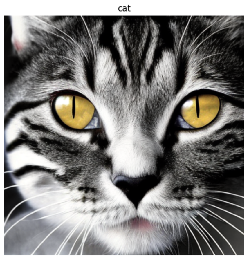
之后,我们可以写 prompt,来验证 endpoint 可以进行推理并可视化。
%%time
import json


response_model = boto3_sm_run_client.invoke_endpoint(
    EndpointName=endpoint_name,
    Body=json.dumps(
        {
            "prompt": "a lovely cat",
        }
    ),
    ContentType="application/json",
)


resp = response_model["Body"].read()


def decode_image(img):
    buff = io.BytesIO(img)
    image = Image.open(buff)
    return image


def display_img_and_prompt(img, prmpt):
    """Display hallucinated image."""
    plt.figure(figsize=(6, 6))
    plt.imshow(np.array(img))
    plt.axis("off")
    plt.title(prmpt)
    plt.show()


display_img_and_prompt(decode_image(resp), "cat")
左滑查看更多
P95 测试
接下来我们进行测试下平均推理时间,执行循环 10 次,取平均值。代码如下:
import numpy as np


results = []
for i in range(0, 10):
    start = time.time()
    prompts = ["Mountains Landscape"]
    response_model = boto3_sm_run_client.invoke_endpoint(
        EndpointName=endpoint_name,
        Body=json.dumps(
            {
                "prompt": "cat",
                "parameters": {}#"text_length": 128}
            }
        ),
        ContentType="application/json",
    )
    results.append((time.time() - start) * 1000)


print("\nPredictions for model latency: \n")
print("\nP95: " + str(np.percentile(results, 95)) + " ms\n")
print("P90: " + str(np.percentile(results, 90)) + " ms\n")
print("Average: " + str(np.average(results)) + " ms\n")
左滑查看更多
Output:
Predictions for model latency:
P95: 2275.67777633667 ms
P90: 2250.3053665161133 ms
Average: 2216.5552616119385 ms
左滑查看更多
总结
Amazon Inferentia2 是一项强大的技术,旨在提高深度学习模型性能并降低推理的成本。与 Amazon Inferentia1 相比,它的性能更高,与其他类似的推理优化 EC2 实例相比,吞吐量提高了 4 倍,延迟降低了 10 倍,性能功耗比提高了 50%。将推理代码迁移到 Amazon Inferentia2 也非常简单直接,它支持的模型广泛,包括大型语言模型和生成 AI 的基础模型。
本文介绍了搭载了 Amazon Inferentia2 芯片的 Inf2 实例在 SageMaker 上部署 Stable Diffusion 模型。读者可以下载源代码自行学习。(https://d1m6v8zdux9m8v.cloudfront.net/SageMaker_INF2_SD21_inference.ipynb)
参考资料
https://awsdocs-neuron.readthedocs-hosted.com/en/latest/index.html
https://github.com/aws-neuron/aws-neuron-sdk
https://aws.amazon.com/ec2/instance-types/inf2/
https://aws.amazon.com/sagemaker/
https://djl.ai/
https://docs.aws.amazon.com/sagemaker/latest/dg/large-model-inference-configuration.html
https://huggingface.co/stabilityai/stable-diffusion-2-1
本篇作者

张铮
亚马逊云科技机器学习产品技术专家,负责基于亚马逊云科技加速计算和 GPU 实例的咨询和设计工作。专注于机器学习大规模模型训练和推理加速等领域,参与实施了国内多个机器学习项目的咨询与设计工作。
赵安蓓
亚马逊云科技解决方案架构师,负责基于亚马逊云平台的解决方案咨询和设计,机器学习 TFC 成员。在数据处理与建模领域有着丰富的实践经验,特别关注医疗领域的机器学习工程化与运用。


听说,点完下面4个按钮
就不会碰到bug了!
