12个必须了解的Pytorch损失函数

损失函数是 ML 模型训练的基础，并且在大多数机器学习项目中，如果没有损失函数，就无法驱动模型做出正确的预测。 通俗地说，损失函数是一种数学函数或表达式，用于衡量模型在某些数据集上的表现。 了解模型在特定数据集上的表现如何，可以让开发人员深入了解在训练期间做出许多决策，例如使用新的、更强大的模型，甚至将损失函数本身更改为不同的类型。 说到损失函数的类型，多年来已经开发了几种损失函数，每种损失函数都适合用于特定的训练任务。

推荐：用 NSDT设计器 快速搭建可编程3D场

在本文中，我们将探索这些不同的损失函数，它们是 PyTorch nn 模块的一部分。 我们将进一步深入探讨 PyTorch 如何通过构建自定义函数将这些损失函数作为其 nn 模块 API 的一部分向用户公开。

现在我们对损失函数是什么有了较高层次的了解，让我们探索一些有关损失函数如何工作的更多技术细节。

1、什么是损失函数？

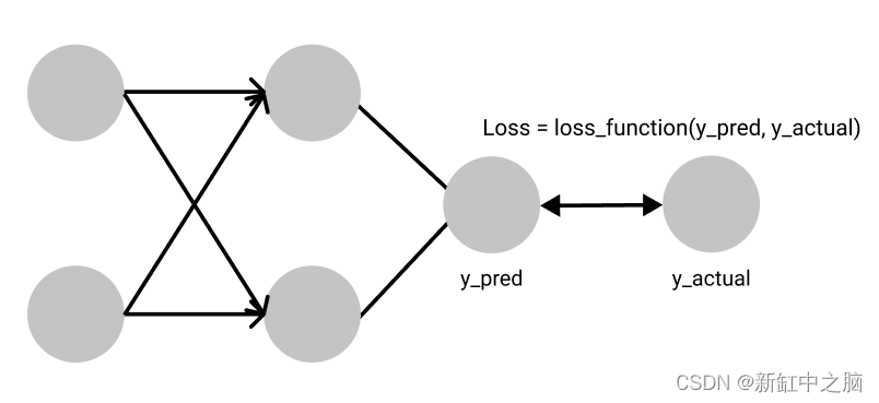
我们之前说过，损失函数告诉我们模型在特定数据集上的表现如何。 从技术上讲，它是通过测量预测值与实际值的接近程度来实现这一点的。 当我们的模型做出的预测非常接近训练和测试数据集的实际值时，这意味着我们有一个非常稳健的模型。

尽管损失函数为我们提供了有关模型性能的关键信息，但这并不是损失函数的主要功能，因为有更强大的技术来评估我们的模型，例如准确性和 F 分数。 损失函数的重要性主要是在训练过程中认识到的，我们在训练中将模型的权重推向最小化损失的方向。 通过这样做，我们增加了模型做出正确预测的概率，如果没有损失函数，这可能是不可能的。

不同的损失函数适合不同的问题，每个损失函数都由研究人员精心设计，以确保训练过程中稳定的梯度流。

有时，损失函数的数学表达式可能有点令人畏惧，这导致一些开发人员将它们视为黑匣子。 稍后我们将揭开 PyTorch 最常用的一些损失函数，但在此之前，让我们先看看如何在 PyTorch 的世界中使用损失函数。

2、PyTorch 中的损失函数

PyTorch 开箱即用，具有许多规范的损失函数和简单的设计模式，使开发人员可以在训练期间非常快速地轻松迭代这些不同的损失函数。 所有 PyTorch 的损失函数都封装在 nn 模块中，这是 PyTorch 所有神经网络的基类。 这使得在项目中添加损失函数就像添加一行代码一样简单。 让我们看看如何在 PyTorch 中添加均方误差损失函数。

import torch.nn as nn
MSE_loss_fn = nn.MSELoss()

从上面的代码返回的函数可用于使用以下格式计算预测与实际值的距离。

#predicted_value is the prediction from our neural network
#target is the actual value in our dataset
#loss_value is the loss between the predicted value and the actual value
Loss_value = MSE_loss_fn(predicted_value, target)

现在我们已经了解了如何在 PyTorch 中使用损失函数，让我们深入了解 PyTorch 提供的几个损失函数的幕后花絮。

3、PyTorch 中有哪些损失函数可用？

PyTorch 附带的许多损失函数大致分为 3 组：回归损失、分类损失和排名损失。

回归损失主要与连续值有关，连续值可以取两个极限之间的任何值。 其中一个例子是对社区房价的预测。

分类损失函数处理离散值，例如将物体分类为盒子、钢笔或瓶子的任务。

排名损失预测值之间的相对距离。 一个例子是人脸验证，我们想知道哪些人脸图像属于特定人脸，并且可以通过根据与目标人脸扫描的相对近似程度对哪些人脸属于和不属于原始人脸持有者进行排名来实现这一点。

4、L1损失函数

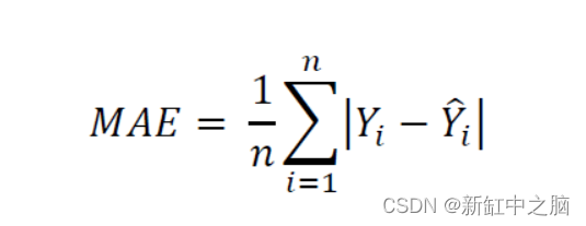
L1 损失函数计算预测张量中每个值与目标张量中每个值之间的平均绝对误差。 它首先计算预测张量中每个值与目标张量中每个值之间的绝对差，并计算每个绝对差计算返回的所有值的总和。 最后，它计算该总和值的平均值以获得平均绝对误差（MAE）。 L1 损失函数对于处理噪声非常稳健。

import torch.nn as nn

#size_average and reduce are deprecated

#reduction specifies the method of reduction to apply to output. Possible values are 'mean' (default) where we compute the average of the output, 'sum' where the output is summed and 'none' which applies no reduction to output

Loss_fn = nn.L1Loss(size_average=None, reduce=None, reduction='mean')

input = torch.randn(3, 5, requires_grad=True)
target = torch.randn(3, 5)
output = loss_fn(input, target)
print(output) #tensor(0.7772, grad_fn=<L1LossBackward>)

返回的单个值是维度为 3 x 5 的两个张量之间的计算损失。

5、均方误差

均方误差与平均绝对误差有一些惊人的相似之处。 它不是像平均绝对误差那样计算预测张量和目标值之间的绝对差，而是计算预测张量和目标张量中的值之间的平方差。 通过这样做，相对较大的差异会受到更多的惩罚，而相对较小的差异会受到较少的惩罚。 然而，MSE 在处理异常值和噪声方面被认为不如 MAE 稳健。

import torch.nn as nn

loss = nn.MSELoss(size_average=None, reduce=None, reduction='mean')
#L1 loss function parameters explanation applies here.

input = torch.randn(3, 5, requires_grad=True)
target = torch.randn(3, 5)
output = loss(input, target)
print(output) #tensor(0.9823, grad_fn=<MseLossBackward>)

6、交叉熵损失

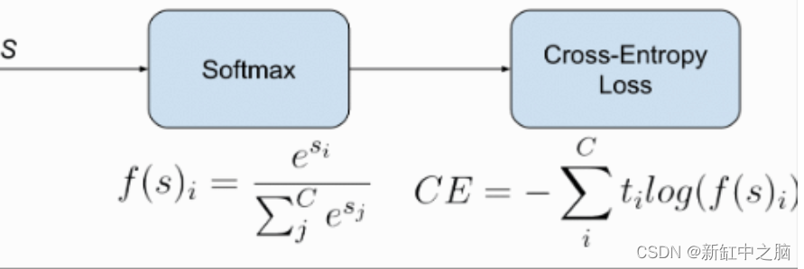
交叉熵损失用于涉及多个离散类的分类问题。 它测量给定随机变量集的两个概率分布之间的差异。 通常，当使用交叉熵损失时，我们网络的输出是一个Softmax层，它确保神经网络的输出是一个概率值（0-1之间的值）。

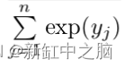
softmax 层由两部分组成 - 特定类别的预测指数。

yi 是特定类别的神经网络的输出。 如果 yi 较大且为负，则此函数的输出是一个接近于零的数字，但绝不会为零；如果 yi 为正且非常大，则该函数的输出接近于 1。

import numpy as np

np.exp(34) #583461742527454.9
np.exp(-34) #1.713908431542013e-15

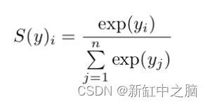
第二部分是归一化值，用于确保softmax层的输出始终是概率值。

这是通过对每个类别值的所有指数求和而获得的。 softmax 的最终方程如下所示：

在 PyTorch 的 nn 模块中，交叉熵损失将 log-softmax 和负对数似然损失合并为单个损失函数。

请注意打印输出中的梯度函数是负对数似然损失 (NLL)。 这实际上揭示了交叉熵损失将 NLL 损失与 log-softmax 层结合起来。

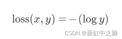
7、负对数似然损失

NLL 损失函数的工作原理与交叉熵损失函数非常相似。 正如前面交叉熵部分提到的，交叉熵损失结合了 log-softmax 层和 NLL 损失来获得交叉熵损失的值。 这意味着通过将神经网络的最后一层设为 log-softmax 层而不是普通的 softmax 层，可以使用 NLL 损失来获得交叉熵损失值。

m = nn.LogSoftmax(dim=1)
loss = nn.NLLLoss()
# input is of size N x C = 3 x 5
input = torch.randn(3, 5, requires_grad=True)
# each element in target has to have 0 <= value < C
target = torch.tensor([1, 0, 4])
output = loss(m(input), target)
output.backward()
# 2D loss example (used, for example, with image inputs)
N, C = 5, 4
loss = nn.NLLLoss()
# input is of size N x C x height x width
data = torch.randn(N, 16, 10, 10)
conv = nn.Conv2d(16, C, (3, 3))
m = nn.LogSoftmax(dim=1)
# each element in target has to have 0 <= value < C
target = torch.empty(N, 8, 8, dtype=torch.long).random_(0, C)
output = loss(m(conv(data)), target)
print(output) #tensor(1.4892, grad_fn=<NllLoss2DBackward>)

#credit NLLLoss — PyTorch 1.9.0 documentation

8、二元交叉熵损失

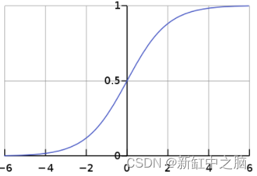
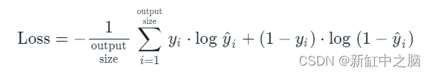
二元交叉熵损失是一类特殊的交叉熵损失，用于将数据点仅分为两类的特殊问题。 此类问题的标签通常是二元的，因此我们的目标是推动模型预测零标签的接近于零的数字和一标签的接近于一的数字。 通常在使用BCE损失进行二元分类时，神经网络的输出是Sigmoid层，以保证输出要么是接近于0的值，要么是接近于1的值。

import torch.nn as nn

m = nn.Sigmoid()
loss = nn.BCELoss()
input = torch.randn(3, requires_grad=True)
target = torch.empty(3).random_(2)
output = loss(m(input), target)
print(output) #tensor(0.4198, grad_fn=<BinaryCrossEntropyBackward>)

9、Logits 的二元交叉熵损失

我在上一节中提到，二元交叉熵损失通常作为 sigmoid 层输出，以确保输出介于 0 和 1 之间。带有 Logits 的二元交叉熵损失将这两层合并为一层。 根据 PyTorch 文档，这是一个数值更稳定的版本，因为它利用了 log-sum exp 技巧。

import torch
import torch.nn as nn

target = torch.ones([10, 64], dtype=torch.float32)  # 64 classes, batch size = 10
output = torch.full([10, 64], 1.5)  # A prediction (logit)
pos_weight = torch.ones([64])  # All weights are equal to 1
criterion = torch.nn.BCEWithLogitsLoss(pos_weight=pos_weight)
loss = criterion(output, target)  # -log(sigmoid(1.5))
print(loss) #tensor(0.2014)

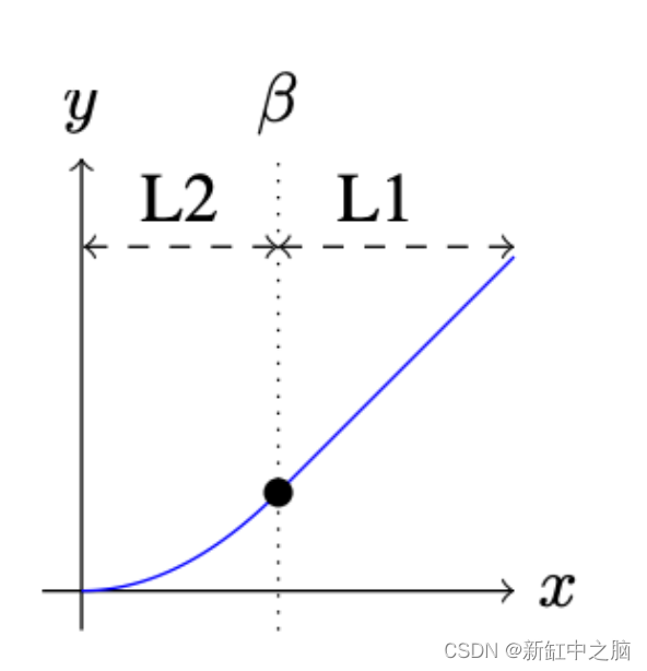
10、平滑 L1 损失

平滑 L1 损失函数通过启发式值 beta 结合了 MSE 损失和 MAE 损失的优点。 Fast R-CNN 论文中介绍了该标准。 当真实值和预测值之间的绝对差值低于 beta 时，该标准使用平方差，就像 MSE 损失一样。 MSE损失的图形是一条连续曲线，这意味着每个损失值处的梯度是变化的并且可以在任何地方导出。 此外，随着损失值的减小，梯度减小，这在梯度下降时很方便。 然而，对于非常大的损失值，梯度爆炸，因此标准切换到平均绝对误差，当绝对差变得大于 beta 并且消除潜在的梯度爆炸时，其梯度对于每个损失值几乎恒定。

import torch.nn as nn

loss = nn.SmoothL1Loss()
input = torch.randn(3, 5, requires_grad=True)
target = torch.randn(3, 5)
output = loss(input, target)

print(output) #tensor(0.7838, grad_fn=<SmoothL1LossBackward>)

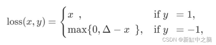
11、Hinge嵌入损耗

Hinge Embedding Loss 主要用于半监督学习任务中，用来衡量两个输入之间的相似度。 当输入张量和包含值 1 或 -1 的标签张量时使用它。 它主要用于涉及非线性嵌入和半监督学习的问题。

import torch
import torch.nn as nn

input = torch.randn(3, 5, requires_grad=True)
target = torch.randn(3, 5)

hinge_loss = nn.HingeEmbeddingLoss()
output = hinge_loss(input, target)
output.backward()

print('input: ', input)
print('target: ', target)
print('output: ', output)

#input:  tensor([[ 1.4668e+00,  2.9302e-01, -3.5806e-01,  1.8045e-01,  #1.1793e+00],
#       [-6.9471e-05,  9.4336e-01,  8.8339e-01, -1.1010e+00,  #1.5904e+00],
#       [-4.7971e-02, -2.7016e-01,  1.5292e+00, -6.0295e-01,  #2.3883e+00]],
#       requires_grad=True)
#target:  tensor([[-0.2386, -1.2860, -0.7707,  1.2827, -0.8612],
#        [ 0.6747,  0.1610,  0.5223, -0.8986,  0.8069],
#        [ 1.0354,  0.0253,  1.0896, -1.0791, -0.0834]])
#output:  tensor(1.2103, grad_fn=<MeanBackward0>)

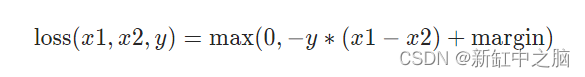
12、边际排名损失

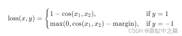
边际排名损失属于排名损失，与其他损失函数不同，其主要目标是测量数据集中一组输入之间的相对距离。 边际排名损失函数采用两个输入和一个仅包含 1 或 -1 的标签。 如果标签为 1，则假设第一个输入应具有比第二个输入更高的排名，如果标签为 -1，则假设第二个输入应具有比第一个输入更高的排名。 这种关系由下面的等式和代码显示。

import torch.nn as nn

loss = nn.MarginRankingLoss()
input1 = torch.randn(3, requires_grad=True)
input2 = torch.randn(3, requires_grad=True)
target = torch.randn(3).sign()
output = loss(input1, input2, target)
print('input1: ', input1)
print('input2: ', input2)
print('output: ', output)

#input1:  tensor([-1.1109,  0.1187,  0.9441], requires_grad=True)
#input2:  tensor([ 0.9284, -0.3707, -0.7504], requires_grad=True)
#output:  tensor(0.5648, grad_fn=<MeanBackward0>)

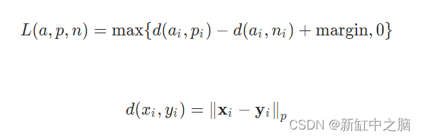
13、三重边际损失

该标准通过使用训练数据样本的三元组来测量数据点之间的相似性。 涉及的三元组是锚样本、正样本和负样本。 目标是1）使正样本和anchor之间的距离尽可能小，2）使anchor和负样本之间的距离大于margin值加上正样本和anchor之间的距离。 通常，正样本与anchor属于同一类，但负样本则不然。 因此，通过使用这个损失函数，我们的目标是使用三元组边缘损失来预测锚点和正样本之间的高相似度值以及锚点和负样本之间的低相似度值。

import torch.nn as nn

triplet_loss = nn.TripletMarginLoss(margin=1.0, p=2)
anchor = torch.randn(100, 128, requires_grad=True)
positive = torch.randn(100, 128, requires_grad=True)
negative = torch.randn(100, 128, requires_grad=True)
output = triplet_loss(anchor, positive, negative)
print(output)  #tensor(1.1151, grad_fn=<MeanBackward0>)

14、余弦嵌入损失

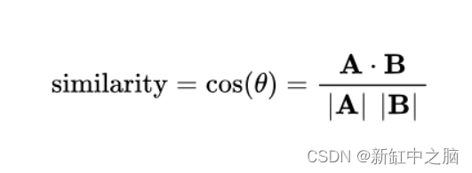
余弦嵌入损失测量给定输入 x1、x2 和包含值 1 或 -1 的标签张量 y 的损失。 它用于测量两个输入的相似或不相似程度。

该标准通过计算空间中两个数据点之间的余弦距离来衡量相似性。 余弦距离与两点之间的角度相关，这意味着角度越小，输入越接近，因此它们越相似。

import torch.nn as nn

loss = nn.CosineEmbeddingLoss()
input1 = torch.randn(3, 6, requires_grad=True)
input2 = torch.randn(3, 6, requires_grad=True)
target = torch.randn(3).sign()
output = loss(input1, input2, target)
print('input1: ', input1)
print('input2: ', input2)
print('output: ', output)

#input1:  tensor([[ 1.2969e-01,  1.9397e+00, -1.7762e+00, -1.2793e-01, #-4.7004e-01,
#         -1.1736e+00],
#        [-3.7807e-02,  4.6385e-03, -9.5373e-01,  8.4614e-01, -1.1113e+00,
#          4.0305e-01],
#        [-1.7561e-01,  8.8705e-01, -5.9533e-02,  1.3153e-03, -6.0306e-01,
#          7.9162e-01]], requires_grad=True)
#input2:  tensor([[-0.6177, -0.0625, -0.7188,  0.0824,  0.3192,  1.0410],
#        [-0.5767,  0.0298, -0.0826,  0.5866,  1.1008,  1.6463],
#        [-0.9608, -0.6449,  1.4022,  1.2211,  0.8248, -1.9933]],
#       requires_grad=True)
#output:  tensor(0.0033, grad_fn=<MeanBackward0>)

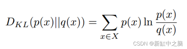
15、Kullback-Leibler 散度损失

给定两个分布 P 和 Q，Kullback Leibler Divergence (KLD) 损失衡量当 P（假设为真实分布）被 Q 替换时丢失了多少信息。通过测量当我们使用 Q 近似 P 时丢失了多少信息，我们能够获得 P 和 Q 之间的相似性，从而驱动我们的算法产生非常接近真实分布 P 的分布。使用 Q 近似 P 时的信息损失与使用 P 近似 Q 时的信息损失不同，因此 KL 散度不对称。

import torch.nn as nn

loss = nn.KLDivLoss(size_average=None, reduce=None, reduction='mean', log_target=False)
input1 = torch.randn(3, 6, requires_grad=True)
input2 = torch.randn(3, 6, requires_grad=True)
output = loss(input1, input2)

print('output: ', output) #tensor(-0.0284, grad_fn=<KlDivBackward>)

16、构建自己的自定义损失函数

PyTorch 为我们提供了两种流行的方法来构建我们自己的损失函数来适应我们的问题； 即使用类实现和使用函数实现。 让我们从函数实现开始看看如何实现这两种方法。

17、自定义损失函数

这是编写自己的自定义损失函数的最简单方法。 它就像创建一个函数、向其传递所需的输入和其他参数、使用 PyTorch 的核心 API 或功能 API 执行某些操作并返回一个值一样简单。 让我们看一下自定义均方误差的演示。

def custom_mean_square_error(y_predictions, target):
  square_difference = torch.square(y_predictions - target)
  loss_value = torch.mean(square_difference)
  return loss_value

在上面的代码中，我们定义了一个自定义损失函数来计算给定预测张量和目标传感器的均方误差

y_predictions = torch.randn(3, 5, requires_grad=True);
target = torch.randn(3, 5)
pytorch_loss = nn.MSELoss();
p_loss = pytorch_loss(y_predictions, target)
loss = custom_mean_square_error(y_predictions, target)
print('custom loss: ', loss)
print('pytorch loss: ', p_loss)

#custom loss:  tensor(2.3134, grad_fn=<MeanBackward0>)
#pytorch loss:  tensor(2.3134, grad_fn=<MseLossBackward>)

我们可以使用自定义损失函数和 PyTorch 的 MSE 损失函数来计算损失，以观察我们是否获得了相同的结果。

18、使用 Python 类自定义损失

这种方法可能是在 PyTorch 中定义自定义损失的标准和推荐方法。 通过对 nn 模块进行子类化，将损失函数创建为神经网络图中的节点。 这意味着我们的自定义损失函数是一个 PyTorch 层，与卷积层完全相同。 让我们看看如何使用自定义 MSE 损失来演示。

class Custom_MSE(nn.Module):
  def __init__(self):
    super(Custom_MSE, self).__init__();

  def forward(self, predictions, target):
    square_difference = torch.square(predictions - target)
    loss_value = torch.mean(square_difference)
    return loss_value
  
  # def __call__(self, predictions, target):
  #   square_difference = torch.square(y_predictions - target)
  #   loss_value = torch.mean(square_difference)
  #   return loss_value

我们可以在“forward”函数调用或“call”内部定义损失的实际实现。 请参阅 Gradient 上的 IPython 笔记本，了解实践中使用的自定义 MSE 函数。

19、结束语

我们已经讨论了很多有关 PyTorch 中可用的损失函数的内容，并且还深入研究了大多数损失函数的内部工作原理。 为特定问题选择正确的损失函数可能是一项艰巨的任务。 希望本教程与官方 PyTorch 文档一起作为尝试了解哪种损失函数最适合您的问题时的指南。

---

原文链接：Pytorch损失函数指南 — BimAnt