k-近邻算法概述
简单地说,k近邻算法采用测量不同特征值之间的距离方法进行分类。
k-近邻算法
- 优点:精度高、对异常值不敏感、无数据输入假定。
- 缺点:计算复杂度高、空间复杂度高。 适用数据范围:数值型和标称型。
k-近邻算法(kNN),它的工作原理是:存在一个样本数据集合,也称作训练样本集,并且样本集中每个数据都存在标签,即我们知道样本集中每一数据与所属分类的对应关系。输入没有标签的新数据后,将新数据的每个特征与样本集中数据对应的特征进行比较,然后算法提取样本集中特征最相似数据(最近邻)的分类标签。一般来说,我们只选择样本数据集中前k个最相似的数据,这就是k-近邻算法中k的出处,通常k是不大于20的整数。最后,选择k个最相似数据中出现次数最多的分类,作为新数据的分类。
k近邻算法的一般流程
- 收集数据:可以使用任何方法。
- 准备数据:距离计算所需要的数值,最好是结构化的数据格式。
- 分析数据:可以使用任何方法。
- 训练算法:此步骤不适用于k近邻算法。
- 测试算法:计算错误率。
- 使用算法:首先需要输入样本数据和结构化的输出结果,然后运行k近邻算法判定输入数据分别属于哪个分类,最后应用对计算出的分类执行后续的处理。
下面将经过编码来了解KNN算法:
import numpy as np
import matplotlib.pyplot as plt
from sklearn import datasets
plt.rcParams['font.sans-serif']=['SimHei'] #用来正常显示中文标签
#准备数据集
iris=datasets.load_iris()
X=iris.data
print('X:\n',X)
Y=iris.target
print('Y:\n',Y)

#处理二分类问题,所以只针对Y=0,1的行,然后从这些行中取X的前两列
x=X[Y<2,:2]
print(x.shape)
print('x:\n',x)
y=Y[Y<2]
print('y:\n',y)
#target=0的点标红,target=1的点标蓝,点的横坐标为data的第一列,点的纵坐标为data的第二列
plt.scatter(x[y==0,0],x[y==0,1],color='red')
plt.scatter(x[y==1,0],x[y==1,1],color='green')
plt.scatter(5.6,3.2,color='blue')
x_1=np.array([5.6,3.2])
plt.title('红色点标签为0,绿色点标签为1,待预测的点为蓝色')
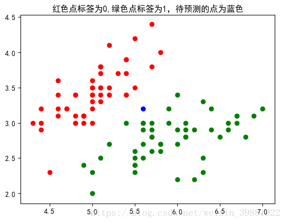
计算完所有点之间的距离后,可以对数据按照从小到大的次序排序。统计距离最近前k个数据点的类别数,返回票数最多的那类即为蓝色点的类别。
#采用欧式距离计算
distances=[np.sqrt(np.sum((x_t-x_1)**2)) for x_t in x]
#对数组进行排序,返回的是排序后的索引
d=np.sort(distances)
nearest=np.argsort(distances)
k=6
topk_y=[y[i] for i in nearest[:k]]
from collections import Counter
#对topk_y进行统计返回字典
votes=Counter(topk_y)
#返回票数最多的1类元素
print(votes)
predict_y=votes.most_common(1)[0][0]
print(predict_y)
plt.show()
Counter({1: 4, 0: 2})
1
从结果可以看出,k=6时,距离蓝色的点最近的6个点钟,有4个属于绿色,2个属于红色,最终蓝色点的标签被预测为绿色。我们将刚才代码中实现的功能可以封装成一个类:
KNN.py
import numpy as np
from collections import Counter
from metrics import accuracy_score
class KNNClassifier:
    def __init__(self,k):
        assert k>=1,'k must be valid'
        self.k=k
        self._x_train=None
        self._y_train=None

    def fit(self,x_train,y_train):
        self._x_train=x_train
        self._y_train=y_train
        return self

    def _predict(self,x):
        d=[np.sqrt(np.sum((x_i-x)**2)) for x_i in self._x_train]
        nearest=np.argsort(d)
        top_k=[self._y_train[i] for i in nearest[:self.k]]
        votes=Counter(top_k)
        return votes.most_common(1)[0][0]

    def predict(self,X_predict):
        y_predict=[self._predict(x1) for x1 in X_predict]
        return np.array(y_predict)

    def __repr__(self):
        return 'knn(k=%d):'%self.k

    def score(self,x_test,y_test):
        y_predict=self.predict(x_test)
        return sum(y_predict==y_test)/len(x_test)
模型选择,将训练集和测试集进行划分
model_selection.py
import numpy as np
def train_test_split(x,y,test_ratio=0.2,seed=None):
    if seed:
        np.random.seed(seed)
    #生成样本随机的序号
    shuffed_indexes=np.random.permutation(len(x))
    print(shuffed_indexes)
    #测试集占样本总数的20%
    test_size=int(test_ratio*len(x))
    test_indexes=shuffed_indexes[:test_size]
    train_indexes=shuffed_indexes[test_size:]
    x_test=x[test_indexes]
    y_test=y[test_indexes]
    x_train=x[train_indexes]
    y_train=y[train_indexes]
    return x_train,x_test,y_train,y_test

'''
sklearn中的train_test_split
from sklearn.model_selection import train_test_split
x_train,x_test,y_train,y_test=tran_test_split(x,y,test_size=0.2,random_state=666)

'''
下面我们采用两种不同的方式吗,对模型的正确率进行衡量
from sklearn import datasets
from sklearn.model_selection import train_test_split
from sklearn.neighbors import KNeighborsClassifier
iris=datasets.load_iris()
x=iris.data
y=iris.target

#sklearn自带的train_test_split
x_train,x_test,y_train,y_test=train_test_split(x,y)
knn_classifier=KNeighborsClassifier(6)
knn_classifier.fit(x_train,y_train)
y_predict=knn_classifier.predict(x_test)
scores=knn_classifier.score(x_test,y_test)
print('acc:{}'.format(sum(y_predict==y_test)/len(x_test)),scores)


#采用我们自己写的
from model_selection import train_test_split
X_train,X_test,y_train,y_test=train_test_split(x,y)
from KNN import KNNClassifier
from metrics import accuracy_score
my_knn=KNNClassifier(k=6)
my_knn.fit(X_train,y_train)
y_predict=my_knn.predict(X_test)
print(accuracy_score(y_test,y_predict))
score=my_knn.score(X_test,y_test)
print(score)
得到正确率之后,想要进一步的提升在测试集上的正确率,我们就需要对模型进行调参
超参数:在算法运行前需要设定的参数(通过领域知识、经验数值、实验搜索来寻找好的超参数)
模型参数:算法过程中学习的参数
在KNN中没有模型参数,KNN算法中的k是典型的超参数,我们将采用实验搜索来寻找好的超参数
寻找最好的k:
def main():
    from sklearn import datasets
    digits=datasets.load_digits()
    x=digits.data
    y=digits.target
    from sklearn.model_selection import train_test_split
    x_train,x_test,y_train,y_test=train_test_split(x,y,test_size=0.2,random_state=666)
    from sklearn.neighbors import KNeighborsClassifier
    # 寻找最好的k
    best_k=-1
    best_score=0
    for i in range(1,11):
        knn_clf=KNeighborsClassifier(n_neighbors=i)
        knn_clf.fit(x_train,y_train)
        scores=knn_clf.score(x_test,y_test)
        if scores>best_score:
            best_score=scores
            best_k=i
    print('最好的k为:%d,最好的得分为:%.4f'%(best_k,best_score))
if __name__ == '__main__':
    main()
最好的k为:4,最好的得分为:0.9917
那么还有没有别的超参数呢?
sklearn中的文档
sklearn.neighbors.KNeighborsClassifier
| Parameters: | n_neighbors : int, optional (default = 5)
weights : str or callable, optional (default = ‘uniform’)
algorithm : {‘auto’, ‘ball_tree’, ‘kd_tree’, ‘brute’}, optional
leaf_size : int, optional (default = 30)
p : integer, optional (default = 2)
metric : string or callable, default ‘minkowski’
metric_params : dict, optional (default = None)
n_jobs : int, optional (default = 1)
|
|---|
- n_neighbors:默认为5,就是k-NN的k的值,选取最近的k个点。
- weights:默认是uniform,参数可以是uniform、distance,也可以是用户自己定义的函数。uniform是均等的权重,就说所有的邻近点的权重都是相等的。distance是不均等的权重,距离近的点比距离远的点的影响大。用户自定义的函数,接收距离的数组,返回一组维数相同的权重。
- algorithm:快速k近邻搜索算法,默认参数为auto,可以理解为算法自己决定合适的搜索算法。除此之外,用户也可以自己指定搜索算法ball_tree、kd_tree、brute方法进行搜索,brute是蛮力搜索,也就是线性扫描,当训练集很大时,计算非常耗时。kd_tree,构造kd树存储数据以便对其进行快速检索的树形数据结构,kd树也就是数据结构中的二叉树。以中值切分构造的树,每个结点是一个超矩形,在维数小于20时效率高。ball tree是为了克服kd树高纬失效而发明的,其构造过程是以质心C和半径r分割样本空间,每个节点是一个超球体。
- leaf_size:默认是30,这个是构造的kd树和ball树的大小。这个值的设置会影响树构建的速度和搜索速度,同样也影响着存储树所需的内存大小。需要根据问题的性质选择最优的大小。
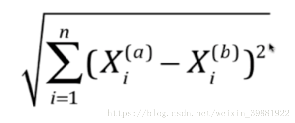
- metric:用于距离度量,默认度量是minkowski,也就是p=2的欧氏距离(欧几里德度量)。
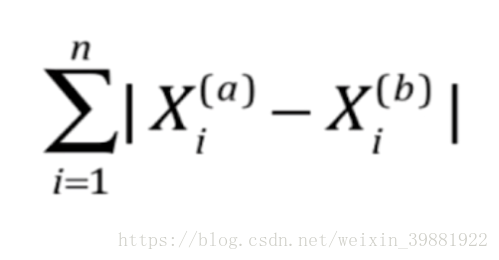
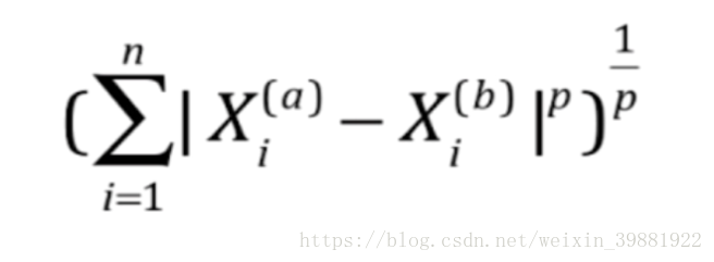
- p:距离度量公式。在上小结,我们使用欧氏距离公式进行距离度量。除此之外,还有其他的度量方法,例如曼哈顿距离。这个参数默认为2,也就是默认使用欧式距离公式进行距离度量。也可以设置为1,使用曼哈顿距离公式进行距离度量。
- metric_params:距离公式的其他关键参数,这个可以不管,使用默认的None即可。
- n_jobs:并行处理设置。默认为1,临近点搜索并行工作数。如果为-1,那么CPU的所有cores都用于并行工作。
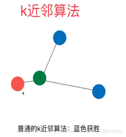
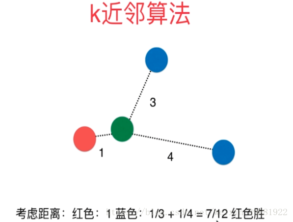
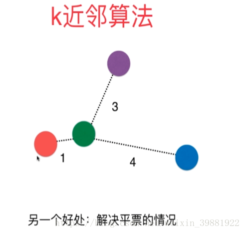
考虑距离?不考虑距离?
当K=3时,如下图所示,由投票法蓝色点胜出,于是绿色的点就归为蓝色点的那一类。但是这样分类我们虽然考虑了离绿色节点最近的三个点,但是却忽略了这三个点到绿色点的距离,从图中可以看出红色的点其实是离绿色的点最近,当我们考虑距离时,我们需要将距离附一个权重值,离得越近,权重越大,通常将距离的导数作为权重:
| 不考虑距离,蓝色点胜 | 考虑距离,红色点胜 |
 |
 |
def main():
    from sklearn import datasets
    digits=datasets.load_digits()
    x=digits.data
    y=digits.target
    from sklearn.model_selection import train_test_split
    x_train,x_test,y_train,y_test=train_test_split(x,y,test_size=0.2,random_state=666)
    from sklearn.neighbors import KNeighborsClassifier
    # 寻找最好的k,weights
    best_k=-1
    best_score=0
    best_method=''
    for method in ['uniform','distance']:
        for i in range(1,11):
            knn_clf=KNeighborsClassifier(n_neighbors=i,weights=method)
            knn_clf.fit(x_train,y_train)
            scores=knn_clf.score(x_test,y_test)
            if scores>best_score:
                best_score=scores
                best_k=i
                best_method=method
    print('最好的k为:%d,最好的得分为:%.4f,最好的方法%s'%(best_k,best_score,best_method))
if __name__ == '__main__':
    main()
| 曼哈顿距离 | 欧式距离 | 明可夫斯基距离 |
 |
 |
 |
对最优的明可夫斯基距离相应的p进行搜索:
def main():
    from sklearn import datasets
    digits=datasets.load_digits()
    x=digits.data
    y=digits.target
    from sklearn.model_selection import train_test_split
    x_train,x_test,y_train,y_test=train_test_split(x,y,test_size=0.2,random_state=666)
    from sklearn.neighbors import KNeighborsClassifier
    # 寻找最好的k,weights
    best_k=-1
    best_score=0
    best_p=-1

    for i in range(1,11):
        for p in range(1,6):
            knn_clf=KNeighborsClassifier(n_neighbors=i,weights='distance',p=p)
            knn_clf.fit(x_train,y_train)
            scores=knn_clf.score(x_test,y_test)
            if scores>best_score:
                best_score=scores
                best_k=i
                best_p=p
    print('最好的k为:%d,最好的得分为:%.4f,最好的p为%d'%(best_k,best_score,best_p))
if __name__ == '__main__':
    main()
最好的k为:3,最好的得分为:0.9889,最好的p为2
GridSearchCV 提供的网格搜索从通过 param_grid 参数确定的网格参数值中全面生成候选。例如,下面的 param_grid:
param_grid = [
  {'C': [1, 10, 100, 1000], 'kernel': ['linear']},
  {'C': [1, 10, 100, 1000], 'gamma': [0.001, 0.0001], 'kernel': ['rbf']},
 ]
探索两个网格的详细解释: 一个具有线性内核并且C在[1,10,100,1000]中取值; 另一个具有RBF内核,C值的交叉乘积范围在[1,10,100,1000],gamma在[0.001,0.0001]中取值。
在本例中:def main():
import numpy as np
from sklearn import datasets
digits=datasets.load_digits()
x=digits.data
y=digits.target
from sklearn.model_selection import train_test_split
x_train,x_test,y_train,y_test=train_test_split(x,y,test_size=0.2,random_state=666)
from sklearn.neighbors import KNeighborsClassifier
#Grid Search定义要搜索的参数
param_grid=[
{
'weights':['uniform'],
'n_neighbors':[i for i in range(1,11)]
},
{
'weights':['distance'],
'n_neighbors':[i for i in range(1,11)],
'p':[i for i in range(1,6)]
}
]
knn_clf=KNeighborsClassifier()
from sklearn.model_selection import GridSearchCV
#n_jobs采用几个核来处理,-1代表计算机有几个核就用几个核进行并行处理,搜索过程中verbose可以进行信息输出,帮助理解搜索状态
grid_search=GridSearchCV(knn_clf,param_grid,n_jobs=-1,verbose=1)
grid_search.fit(x_train,y_train)
#返回网格搜索最佳分类器
print(grid_search.best_estimator_)
#返回网格搜索最佳分类器的参数
print(grid_search.best_params_)
#返回网格搜索最佳分类器的分数
print(grid_search.best_score_)
knn_clf=grid_search.best_estimator_
print(knn_clf.score(x_test,y_test))
if __name__ == '__main__':
main()
Fitting 3 folds for each of 60(10+50) candidates, totalling 180 fits
[Parallel(n_jobs=-1)]: Done  34 tasks      | elapsed:    1.6s
[Parallel(n_jobs=-1)]: Done 180 out of 180 | elapsed:   30.6s finished
KNeighborsClassifier(algorithm='auto', leaf_size=30, metric='minkowski',
           metric_params=None, n_jobs=1, n_neighbors=3, p=3,
           weights='distance')
{'n_neighbors': 3, 'weights': 'distance', 'p': 3}
0.985386221294
0.983333333333
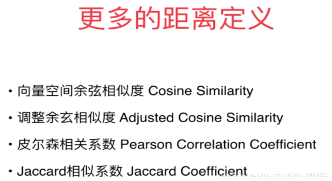
在衡量距离时,其实还有一个非常重要的概念就是数据归一化Feature Scaling
| 肿瘤大小(厘米) | 发现时间(天) | |
| 样本1 | 1 | 200=0.55年 |
| 样本2 | 5 | 100=0.27年 |
解决方案:将所有的数据映射同一尺度
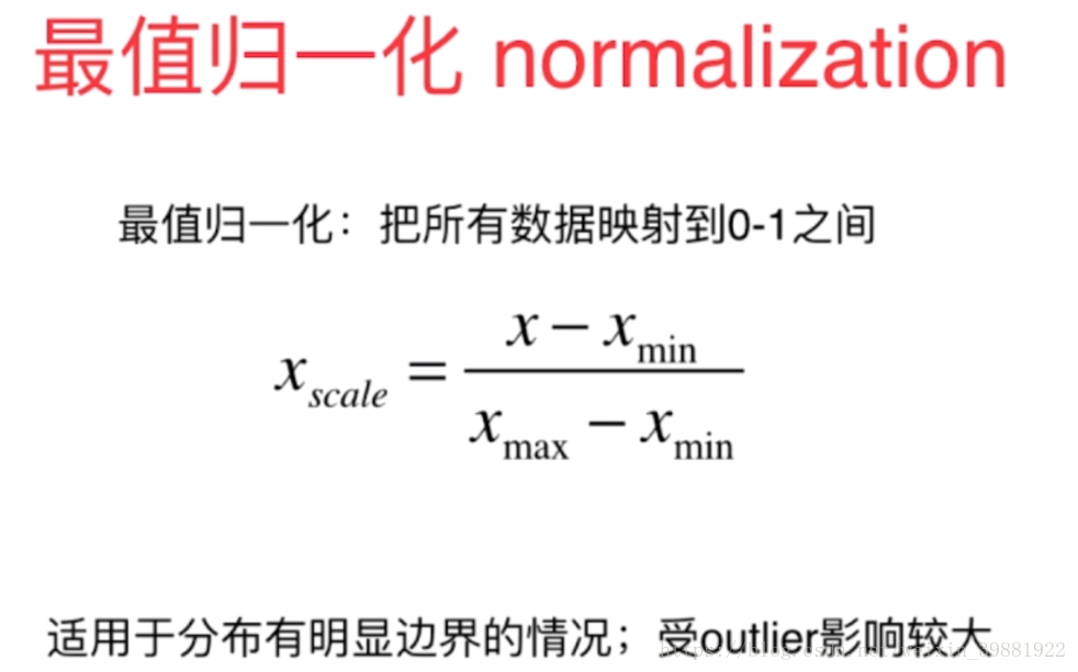
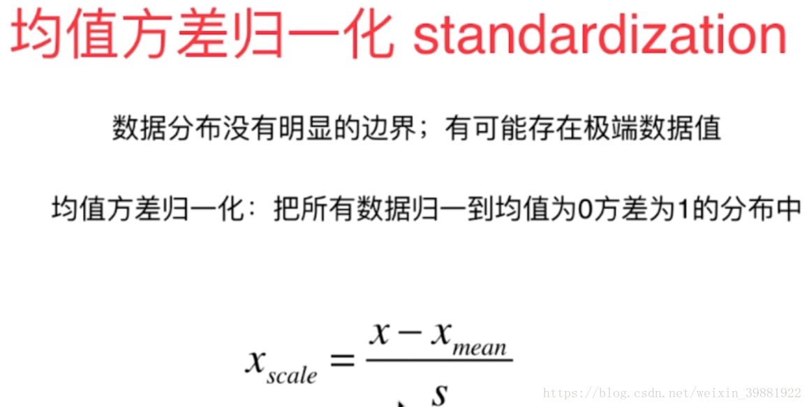
import numpy as np
import matplotlib.pyplot as plt
#最值归一化
x=np.random.randint(0,100,size=100)
print(x)
normal_x=(x-np.min(x))/(np.max(x)-np.min(x))
print(normal_x)
#均值方差归一化
x2=np.random.randint(0,100,(50,2))
print(x2)
x2=np.array(x2,dtype=float)
x2[:,0]=(x2[:,0]-np.mean(x2[:,0]))/np.std(x2[:,0])
x2[:,1]=(x2[:,1]-np.mean(x2[:,1]))/np.std(x2[:,1])
plt.scatter(x2[:,0],x2[:,1])
plt.show()
x:[49 27 88 47  6 89  9 98 17 72 46 46 80 62 28 38  0 27 22 14  2 79 70 73 15
 57 85  6 11 76 59 62 23 32 82 78  0 45  8 82 13 81 99 61 43 21 45 61 93 63
 66 57 78 60 50  8 29 63 74  8 25 55 10 69  3 77 41 24 15 23 21 31 36 78 94
 52 12  1 23 99  8 12 15 37 75 75 27 14 31 75  6 56 29 96 23  0 22 98 86 10]
normal_x:[ 0.49494949  0.27272727  0.88888889  0.47474747  0.06060606  0.8989899
  0.09090909  0.98989899  0.17171717  0.72727273  0.46464646  0.46464646
  0.80808081  0.62626263  0.28282828  0.38383838  0.          0.27272727
  0.22222222  0.14141414  0.02020202  0.7979798   0.70707071  0.73737374
  0.15151515  0.57575758  0.85858586  0.06060606  0.11111111  0.76767677
  0.5959596   0.62626263  0.23232323  0.32323232  0.82828283  0.78787879
  0.          0.45454545  0.08080808  0.82828283  0.13131313  0.81818182
  1.          0.61616162  0.43434343  0.21212121  0.45454545  0.61616162
  0.93939394  0.63636364  0.66666667  0.57575758  0.78787879  0.60606061
  0.50505051  0.08080808  0.29292929  0.63636364  0.74747475  0.08080808
  0.25252525  0.55555556  0.1010101   0.6969697   0.03030303  0.77777778
  0.41414141  0.24242424  0.15151515  0.23232323  0.21212121  0.31313131
  0.36363636  0.78787879  0.94949495  0.52525253  0.12121212  0.01010101
  0.23232323  1.          0.08080808  0.12121212  0.15151515  0.37373737
  0.75757576  0.75757576  0.27272727  0.14141414  0.31313131  0.75757576
  0.06060606  0.56565657  0.29292929  0.96969697  0.23232323  0.
  0.22222222  0.98989899  0.86868687  0.1010101 ]

 |
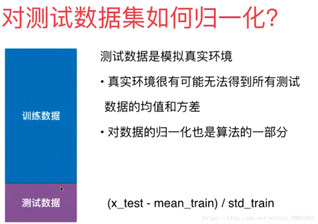 |
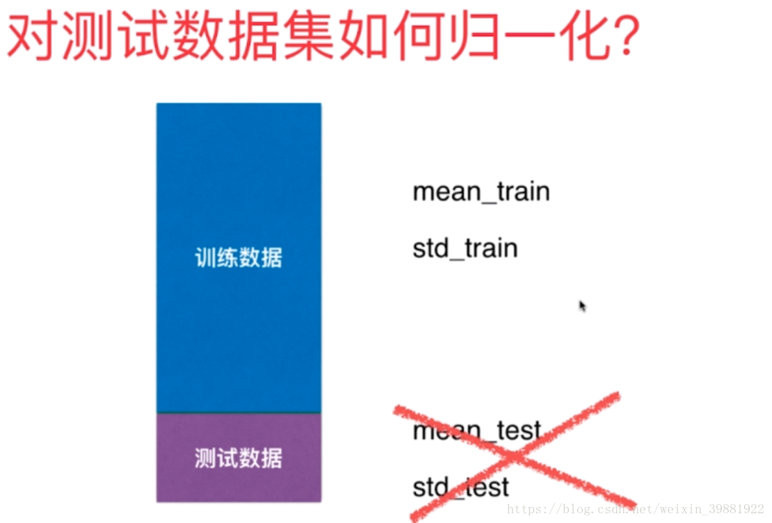
from sklearn.model_selection import train_test_split
x_train,x_test,y_train,y_test=train_test_split(x,y,test_size=0.2,random_state=666)
#sklearn中的StandardScaler
from sklearn.preprocessing import StandardScaler
standardscaler=StandardScaler()
standardscaler.fit(x_train)
#均值
print(standardscaler.mean_)
#方差
print(standardscaler.scale_)
x_train_standard=standardscaler.transform(x_train)
x_test_standard=standardscaler.transform(x_test)
print(x_train_standard)
from sklearn.neighbors import KNeighborsClassifier
knn_clf=KNeighborsClassifier(n_neighbors=3)
knn_clf.fit(x_train_standard,y_train)
scores=knn_clf.score(x_test_standard,y_test)
print(scores)
总结:
| 优点 | 不足 |
解决分类问题 天然可以解决多分类问题 思想简单,效果强大 |
最大缺点:效率低下,如果训练集有m个样本,n个特征,则预测每一个新的数据,需要O(m*n) 维度灾难,随着维度的增加,‘看似相近’的两个点之间的距离会越来越大 缺点2:数据高度相关 缺点3:预测结果不具有可解释性 |
此外,使用K近邻算法还可以解决回归问题,预测房价,成绩等。用平均距离预测