1 Getting Started
1.1 What is NumPy?
NumPy is the fundamental package for scientific computing in Python.
总之,各种各样的计算
Numpy的核心是ndarry object
There are several important differences between NumPy arrays and the standard Python sequences:(和Python的一些差异)
NumPy数组在创建时具有固定的大小,这与Python列表List(可以动态增长)不同。更改ndarray的大小将创建一个新数组并删除原始数组。
NumPy数组中的元素都需要具有相同的数据类型,因此在内存中的大小相同。例外:可以有(Python,包括NumPy)对象的数组,从而允许不同大小元素的数组。
NumPy数组便于对大量数据进行高级数学运算和其他类型的运算。通常,与使用Python的内置序列相比,这样的操作执行效率更高,代码更少。
越来越多的基于科学和数学Python的软件包正在使用NumPy数组;尽管这些通常支持Python序列输入,但它们在处理之前将这些输入转换为NumPy数组,并且通常输出NumPy阵列。换句话说,为了有效地使用当今基于Python的科学/数学软件,仅仅知道如何使用Python的内置序列类型是不够的,还需要知道如何使用NumPy数组。
在Numpy中, element-by-element operations are the “default mode” when an ndarray is involved【当数组包括其中时,元素对应相乘为默认格式】
c = a * b
1.2 Why is NumPy Fast?
Vectorization【矢量化】
Broadcasting【广播机制】
2 NumPy quickstart
2.1 The Basics
NumPy的主要对象是相同结构的多维数组
它是一个由相同类型的元素(通常是数字)组成的表,由非负整数元组作为索引
在NumPy中,dimensions被称为轴axes
[1, 2, 1]	# one axis,a length of 3
# the array has 2 axes,he first axis has a length of 2, the second axis has a length of 3.第一个维度是行,第二个维度是列
[[1., 0., 0.],
 [0., 1., 2.]]
NumPy’s array class is called ndarray
注意:numpy.array is not the same as the Standard Python Library class array.array
Python 中array.array只能处理one-dimensional arrays
an ndarray object重要的属性:
# 1 ndarray.ndim:the number of axes (dimensions) of the array【维度的数量】
# 2 ndarray.shape:the dimensions of the array.This is a tuple of integers indicating the size of the array in each dimension.
For a matrix with n rows and m columns, shape will be (n,m). The length of the shape tuple is therefore the number of axes, ndim.
【数组的维度。这是一个整数元组,表示每个维度中数组的大小。
对于一个有n行m列的矩阵,shape将是(n,m)
因此,the shape tuple的长度就是轴的数量ndim】
# 3 ndarray.size:the total number of elements of the array.
This is equal to the product of the elements of shape.
【数组中所有元素的个数,等于array shape所有元素的乘积】
# 4 ndarray.dtype:an object describing the type of the elements in the array.
One can create or specify dtype’s using standard Python types.
Additionally NumPy provides types of its own. numpy.int32, numpy.int16, and numpy.float64 are some examples.
【描述数组中元素类型的对象
可以使用标准Python类型创建或指定dtype。
此外,NumPy还提供了自己的类型。比如numpy.int32、numpy.int16和numpy.float64】
# 4 ndarray.itemsize:the size in bytes of each element of the array.
For example, an array of elements of type float64 has itemsize 8 (=64/8),
while one of type complex32 has itemsize 4 (=32/8).
It is equivalent to 【ndarray.dtype.itemsize】
【数组中每个元素的大小(以字节为单位)。
例如,float64类型(64 bit)的元素数组的项大小为8(=64/8),
而complex32(32 bit)类型的元素阵列的项大小是4(=32/8)
它相当于ndarray.dtype.itemsize】
# 5 ndarray.data:the buffer containing the actual elements of the array. Normally, we won’t need to use this attribute because we will access the elements in an array using indexing facilities.
【该缓冲区包含数组的实际元素。
通常,我们不需要使用此属性,因为我们将使用索引功能访问数组中的元素。】
2.1.1 A Example
import numpy as np
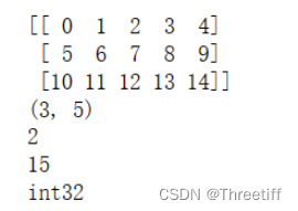
a = np.arange(15).reshape(3, 5)
print(a)
print(a.shape)
print(a.ndim)
print(a.size)
print(a.dtype)
type(a)
# numpy.ndarray
b = np.array([3,4,5])
type(b)
# numpy.ndarray
2.1.2 Array Creation【数组创建】
存在几种方法新建数组:
- 使用
array()函数从常规Python列表或元组创建数组。从序列中的元素的类型推导得到的数组的类型
import numpy as np
a = np.array([2, 3, 4])		# [2, 3, 4]是一个列表
a
a.dtype
一个常见的错误是调用具有多个参数的数组,而不是提供单个序列作为参数【如果使用列表,一定不能忘记中括号[]】
a = np.array(1, 2, 3, 4)    # WRONG
Traceback (most recent call last):
  ...
TypeError: array() takes from 1 to 2 positional arguments but 4 were given
a = np.array([1, 2, 3, 4])  # RIGHT
array()可将sequences of sequences【序列的序列】转换为two-dimensional arrays
可将sequences of sequences of sequences【序列的序列的序列】转换为three-dimensional arrays
b = np.array([(1,2,3),(4,5,6)])	# 最外面是方括号[],一个列表中包含了两个元组
b
array([[1, 2, 3],
    [4, 5, 6]])
同时,也可以进行数组类型的转换
c = np.array([[1, 2], [3, 4]], dtype=complex)
c
array([[1.+0.j, 2.+0.j],
       [3.+0.j, 4.+0.j]])
通常,数组的元素最初是未知的,但其大小是已知的。
因此,NumPy提供了几个函数来创建具有初始占位符内容的数组
# zeros:creates an array full of zeros【全是0】
# ones:creates an array full of ones【全是1】
# empty:initial content is random,depends on the state of the memory【初始内容随机,取决于内存的状态】
# 默认,the dtype of the created array is float64,但可以通过关键字dtype进行更改

a = np.zeros((2,5))
a
array([[0., 0., 0., 0., 0.],
       [0., 0., 0., 0., 0.]])
b = np.ones((2,3,5), dtype=np.int16)
b
array([[[1, 1, 1, 1, 1],
        [1, 1, 1, 1, 1],
        [1, 1, 1, 1, 1]],

       [[1, 1, 1, 1, 1],
        [1, 1, 1, 1, 1],
        [1, 1, 1, 1, 1]]], dtype=int16)
c = np.empty((2,4))
c
array([[0.00000000e+000, 0.00000000e+000, 0.00000000e+000,
        0.00000000e+000],
       [0.00000000e+000, 8.61650486e-321, 1.78019082e-306,
        8.90103559e-307]])
为了创建数字序列,利用arange(和Python中range类似),但arange返回一个数组
a = np.arange(10,30,5)	# 10是start,30是end,5是interval【间隔】
a
array([10, 15, 20, 25])
b = np.arange(0,2,0.6)	# end可以不达到,interval可以是小数
b
array([0. , 0.6, 1.2, 1.8])
当arange与浮点型参数一起使用时,不太好预测最终数组中元素的数量
因此,更加推荐linspace,可以让我们设置数组中元素的数量
from numpy import pi
a = np.linspace(0,2,9)	# 从0到2的9个数,包括0和2,均匀分配
a
array([0.  , 0.25, 0.5 , 0.75, 1.  , 1.25, 1.5 , 1.75, 2.  ])
2.1.3 Printing Arrays 【打印数组】
当打印数组,NumPy displays it in a similar way to nested lists【和Lists类似】
最后一个轴是从左到右打印的【从左到右读一行】
倒数第二个是从上到下打印的【从上到下读一列】
其余部分也从上到下打印,每一个slice与下一个slice用空行隔开
一维数组打印为行【row】
二维数组打印为矩阵【matrix】
三维数组打印为矩阵的Lists
如果想要强制Numpy打印所有数组,使用np.set_printoptions更改打印选项
# 全部输出
np.set_printoptions(threshold=sys.maxsize)  # sys module should be imported
2.1.4 Basic Operations
数组运算按照元素elementwise进行【按元素进行】,将创建一个新的数组
a = np.array([20, 30, 40, 50])
b = np.arange(4)
b
c = a - b
与许多矩阵语言不同,乘积运算符*在NumPy数组中按元素操作。
矩阵乘积matrix product可以使用@运算符(在python中>=3.5)或the dot function or method
a = np.array([[1,1],[0,1]])
b = np.array([[2,0],[3,4]])

print(a*b)	# 对应元素相乘
print(a@b)	# 矩阵乘法
print(a.dot(b))	# 矩阵乘法
# 结果如下:
[[2 0]
 [0 4]]
[[5 4]
 [3 4]]
[[5 4]
 [3 4]]
这些运算如+=或者*=,直接对原数组进行处理,不创建新数组
rg = np.random.default_rng(1)	# 设置随机树生成器,数字可以更改
a = np.ones((2, 3), dtype=int)
print(a)
[[1 1 1]
 [1 1 1]]
b = rg.random((2,3))
[[0.51182162 0.9504637  0.14415961]
 [0.94864945 0.31183145 0.42332645]]
print(b)
b +=a	# 对b进行处理,等同于b=b+a
print(b)
[[1.51182162 1.9504637  1.14415961]
 [1.94864945 1.31183145 1.42332645]]
 # 但是a = a + b,b不能自动从float转为int
 a += b
 # UFuncTypeError: Cannot cast ufunc 'add' output from dtype('float64') to dtype('int32') with casting rule 'same_kind'
当使用不同类型的数组进行操作时,生成的数组的类型对应于更通用或更精确【more general or precise one】的数组(一种称为向上投射的行为)
a = np.ones(3, dtype=np.int32)	# 'int32'
b = np.linspace(0, pi, 3)
b.dtype.name	# 'float64'
c = a + b
c.dtype.name	# 'float64'
许多一元运算,例如计算数组中所有元素的和,都是作为ndarray类的方法method实现的
a = rg.random((2,3))
print(a)
print(a.sum())
print(a.max())
print(a.min())
# 结果如下:
[[0.32973172 0.7884287  0.30319483]
 [0.45349789 0.1340417  0.40311299]]
2.412007822394087
0.7884287034284043
0.13404169724716475
默认情况下,无论数组的形状如何,这些操作都应用于数组,就好像它是一个数字列表一样【 a list of numbers】
但是,通过指定axis参数,可以沿array的指定axis应用操作:
axis=0:对列进行处理
axis=1:对行进行处理
# 指定轴参数axis
b = np.arange(12).reshape(3,4)
print(b)
[[ 0  1  2  3]
 [ 4  5  6  7]
 [ 8  9 10 11]]
print(b.sum(axis=0))	# 每列求和
[12 15 18 21]
print(b.min(axis=1))	# 每行求最小
[0 4 8]
print(b.cumsum(axis=1))	# 每行元素依次累加,得到和原来完全相同的数组
[[ 0  1  3  6]
 [ 4  9 15 22]
 [ 8 17 27 38]]
print(b.cumsum(axis=0))	# 每列元素依次累加,得到和原来完全相同的数组
[[ 0  1  2  3]
 [ 4  6  8 10]
 [12 15 18 21]]
2.1.5 Universal Functions【常见函数】
NumPy提供了熟悉的数学函数,如sin、cos和exp
Numpy中将这些函数设置为universal functions(ufunc)
在使用这些函数时,按元素运算,生成数组作为输出
b = np.arange(3)
print(np.exp(b))
[1.         2.71828183 7.3890561 ]
print(np.sqrt(b))
[0.         1.         1.41421356]
2.1.6 Indexing, Slicing and Iterating【索引、切片、迭代】
一维数组可以被索引、切片和迭代,就像 lists and other Python sequences一样
a = np.arange(10)**3	# **是幂的意思
print(a)
[  0   1   8  27  64 125 216 343 512 729]
print(a[2])		# 从0开始
8
print(a[2:5])	# 切片
[ 8 27 64]
a[:6:2] = 1000	# 从开始到索引6(不包括索引6),间隔为2,每隔2个元素设置为1000
print(a)
[1000    1 1000   27 1000  125  216  343  512  729]
print(a[::-1])	# 两个冒号代表从开始到结尾|将数组a反转,注意,对a本身没有什么影响,除非重新赋值一个新数组
[ 729  512  343  216  125 1000   27 1000    1 1000]
多维数组每个轴可以有一个索引。这些索引以逗号分隔的元组形式给出:
def f(x,y):
    return 10*x+y

# fromfunction():通过f,创建特定的数组
b = np.fromfunction(f, (5, 4), dtype=int)	# (5,4)指数组的shape,x从0-4,y从0-3
b
array([[ 0,  1,  2,  3],
       [10, 11, 12, 13],
       [20, 21, 22, 23],
       [30, 31, 32, 33],
       [40, 41, 42, 43]])
print(b[2,3])
print(b[0:5, 1])	# 0-5(不包括5)行,第2列
print(b[:, 1])	# 所有行,第2列
print(b[1:3, :] )	# 所有列,1-3行
当提供的索引少于轴的数量时,缺失的索引被视为完整切片:
b[-1]等同于b[-1, :]【最后一列,所有行】
b[i]的i后面可以跟冒号:或者dots...
dots(…)代表生成完整索引元组所需的冒号
意思就是:把需要的冒号通过…表示
# if x is an array with 5 axes
x[1, 2, ...] is equivalent to x[1, 2, :, :, :],
x[..., 3] to x[:, :, :, :, 3] and
x[4, ..., 5, :] to x[4, :, :, 5, :]
# 例子
c = np.array([[[  0,  1,  2],  # a 3D array (two stacked 2D arrays)
               [ 10, 12, 13]],
              [[100, 101, 102],
               [110, 112, 113]]])
print(c)
[[[  0   1   2]
  [ 10  12  13]]
 [[100 101 102]
  [110 112 113]]]
print(c.shape)	# (2, 2, 3)
print(c[1,...])	# same as c[1, :, :] or c[1]【第二个块】
[[100 101 102]
 [110 112 113]]
print(c[...,2])	# same as c[:, :, 2]【第3列】
[[  2  13]
 [102 113]]
在多维数组上的迭代是相对于第一个轴完成的:
def f(x,y):
    return 10*x+y
b = np.fromfunction(f, (5, 4), dtype=int)	# (5,4)指数组的shape,x从0-4,y从0-3
b
array([[ 0,  1,  2,  3],
       [10, 11, 12, 13],
       [20, 21, 22, 23],
       [30, 31, 32, 33],
       [40, 41, 42, 43]])
for row in b:
    print(row)	# 按行读取
# 结果如下:
[0 1 2 3]
[10 11 12 13]
[20 21 22 23]
[30 31 32 33]
[40 41 42 43]
然而,如果要对数组中的每个元素执行操作,可以使用展开flat属性,该属性是an iterator over all the elements of the array:
for element in b.flat:
    print(element)
# 结果
0
1
2
3
10
11
12
13
20
21
22
23
30
31
32
33
40
41
42
43
2.2 Shape Manipulation【形状管理】
2.2.1 Changing the shape of an array
阵列的shape由沿每个轴的元素数量给定:
rg = np.random.default_rng(1)
a = np.floor(10*rg.random((3,4)))	# 下取整
a
array([[5., 9., 1., 9.],
       [3., 4., 8., 4.],
       [5., 0., 7., 5.]])
a.shape
(3, 4)
阵列的形状可以通过各种命令进行更改。请注意,以下三个命令都返回一个修改后的数组,但不会更改原始数组:
print(a.ravel(),a.ravel().shape)	# 展开flattened

print(a.reshape(6, 2))	# 6行2列,进行形状重设,各维度的乘积需保持不变
[[5. 9.]
 [1. 9.]
 [3. 4.]
 [8. 4.]
 [5. 0.]
 [7. 5.]]
print(a.T, a.T.shape)	# 转置[4,3]
[[5. 3. 5.]
 [9. 4. 0.]
 [1. 8. 7.]
 [9. 4. 5.]]
 (4, 3)
ndarray.resize method modifies the array itself【改变自身shape】
a.resize((2,6))
a
在reshape上,如果出现-1,那么,自动计算该维度的size
a.reshape(3, -1)
# 3行,自动计算列数12/3=4列
2.2.2 Stacking together different arrays
几个array可以沿着不同的轴堆叠在一起:
- vstack():【行堆叠,行数增加】
- hstack():【列堆叠,列数增加】
a = np.floor(10 * rg.random((2, 2)))
b = np.floor(10 * rg.random((2, 2)))
print(a)
[[5. 9.]
 [1. 9.]]
print(b)
[[3. 4.]
 [8. 4.]]
c = np.vstack((a, b))	# vstack进行行堆叠
print(c)
[[5. 9.]
 [1. 9.]
 [3. 4.]
 [8. 4.]]
d = np.hstack((a, b))	# hstack进行列堆叠
[[5. 9. 3. 4.]
 [1. 9. 8. 4.]]
print(d)
- column_stack():【对于1D数组,按列堆叠-列数增加,和hstack()不同】【对于2D数组,和hstack()相同】
- row_stack():【进行行堆叠】
对于函数column_stack:将 1D arrays按照列堆叠为2D array
# column_stack对于二维数组而言,进行列的堆叠
e = np.column_stack((a, b))
[[5. 9. 3. 4.]
 [1. 9. 8. 4.]]

a = np.array([4., 2.])
b = np.array([3., 8.])
c = np.column_stack((a, b)) # column_stack对于一维数组而言,将一维数据看作列,返回二维数组
[[4. 3.]
 [2. 8.]]
d = np.hstack((a, b))	# 由于a和b都只有一列,生成的d也是一列
print(d)
 [4. 2. 3. 8.]
利用newaxis
from numpy import newaxis

a = np.array([4., 2.])
a = a[:, newaxis]	# 将a看作一个2维的矢量
array([[4.],
       [2.]])	# 4外面存在两个中括号
c = np.column_stack((a[:, newaxis], b[:, newaxis]))	# 按照列堆叠
array([[4., 3.],
       [2., 8.]])
d = np.hstack((a[:, newaxis], b[:, newaxis]))	# 按照行堆叠
d
array([[4., 3.],
       [2., 8.]])
# 上述两种方法结果一样
对于函数row_stack,对于任何输入数组,都与vstack相同
事实上,row_stack是vstack的别名
np.column_stack is np.hstack
False	# 两者不相同
np.row_stack is np.vstack
True	# 两者相同
总之,对于二维以上的arrays
hstack沿their second axes进行堆叠【horizontal】
vstack沿their first axes进行堆叠【vertical】
concatenate进行给定编号轴的连接
注意:在复杂情况下,r_和c_可用于通过沿一个轴堆叠数字来创建array。They allow the use of range literals:
a = np.r_[1:4, 0, 4]
a
array([1, 2, 3, 0, 4])

# hstack, vstack, column_stack, concatenate, c_, r_ 这些比较类似
当与数组一起用作参数时,r_和c_在默认行为上类似于vstack和hstack,但允许使用一个可选参数,给出要连接的轴的编号
2.2.3 Splitting one array into several smaller ones【数组拆分】
hsplit可以沿array的水平轴拆分array(方法1:指定要返回的等形状数组的数量|方法2:指定应该进行分割的列)
a = np.floor(10 * rg.random((2, 12)))
print(a)
[[5. 9. 1. 9. 3. 4. 8. 4. 5. 0. 7. 5.]
 [3. 7. 3. 4. 1. 4. 2. 2. 7. 2. 4. 9.]]
b = np.hsplit(a,3)	# 按照列进行分割,分为3份
print(b)
[array([[5., 9., 1., 9.],[3., 7., 3., 4.]]),
array([[3., 4., 8., 4.],[1., 4., 2., 2.]]),
array([[5., 0., 7., 5.],[7., 2., 4., 9.]])]
c = np.hsplit(a, (3, 4))	# 指定要分割的列通过括号实现,在第3列和第4列分别进行分割【第3列之前|3-4列|第4列之后,总共分为3份】
print(c)
[array([[5., 9., 1.],[3., 7., 3.]]),
array([[9.],[4.]]),
array([[3., 4., 8., 4., 5., 0., 7., 5.],[1., 4., 2., 2., 7., 2., 4., 9.]])]
vsplit沿着垂直轴【vertical axis】进行分割
array_split允许选择特定的轴进行分割
2.3 Copies and Views【复制】
在操作和操作数组时,有时会将其数据复制到新数组中,有时则不会。有三种情况:
2.3.1 No Copy at All【不复制】
简单的指定不会复制对象或其数据
a = np.array([[ 0,  1,  2,  3],
              [ 4,  5,  6,  7],
              [ 8,  9, 10, 11]])
b = a	# 没有创建新的object
True
b is a	# a和b是同一数组object的两个命名
2.3.2 View or Shallow Copy【浅复制】
不同的数组对象可以共享相同的数据。view方法创建一个新的数组对象,用于查看相同的数据
c = a.view()
c is a	# c和a不同
False
2.3.3 Deep Copy【深复制】
copy方法对数组和数据进行完整的复制
d = a.copy()	# 包括新数据的新数组被创建
d is a	# d和a不共享任何数据
False
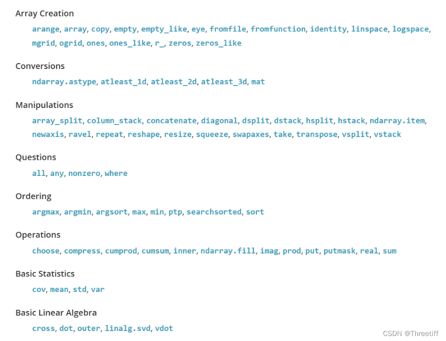
2.3.4 Functions and Methods Overview【函数和方法预览】
2.4 Less Basic
2.4.1 Broadcasting rules【广播原则】
广播允许通用函数以有意义的方式处理shape不完全相同的输入
- 第一条规则:如果所有输入数组的维数不相同,则会重复为较小数组的shape加上“1”,直到所有数组的维数相同。
- 第二条规则:确保沿特定维度大小为1的array的行为,就好像它们具有沿着该维度拥有最大shape的array的size一样。假设数组元素的值与“广播”数组的维度相同。
在应用广播规则之后,所有array的大小一定会匹配
2.5 Advanced indexing and index tricks
NumPy提供了比常规Python序列更多的indexing功能。
除了通过整数和切片【integers and slices】进行索引外,正如我们之前看到的,数组还可以通过【整数数组和布尔数组】进行索引。
2.5.1 Indexing with Arrays of Indices【数组索引】
a = np.arange(12)**2
i = np.array([1, 1, 3, 8, 5]) 	# 索引构成的数组
a[i]	# i指数组的下标
array([ 1,  1,  9, 64, 25], dtype=int32)
j = np.array([[3, 4], [9, 7]])	# 二维数组
a[j]	# 得到的数组与j的shape相同
array([[ 9, 16],
       [81, 49]], dtype=int32)
当索引数组a是多维时,单个索引数组指的是a的第一个维度
以下示例通过使用调色板将标签图像转换为彩色图像来显示此行为
# 调色板
palette = np.array([[0, 0, 0],         # black
                    [255, 0, 0],       # red
                    [0, 255, 0],       # green
                    [0, 0, 255],       # blue
                    [255, 255, 255]]) 	# black
image = np.array([[0, 1, 2, 0],
                  [0, 3, 4, 0]])	# 相当于索引数组(2, 4),每个数字代表调色板上的颜色
palette[image]	# 得到的结果与image的shape相同,并且由于palette内每个元素是三维,最终数组shape为(2, 4, 3)
array([[[  0,   0,   0],
        [255,   0,   0],
        [  0, 255,   0],
        [  0,   0,   0]],

       [[  0,   0,   0],
        [  0,   0, 255],
        [255, 255, 255],
        [  0,   0,   0]]])
还可以为【多个维度】提供索引。但每个维度的索引数组必须具有相同的形状。
a = np.arange(12).reshape(3, 4)
array([[ 0,  1,  2,  3],
       [ 4,  5,  6,  7],
       [ 8,  9, 10, 11]])
i = np.array([[0, 1], [1, 2]]) # indices for the first dim of `a`【a的第一个维度的索引】
j = np.array([[2, 1], [3, 3]]) # indices for the second dim of `a`【a的第二个维度的索引】
a[i,j]	# i和j的shape必须相同
array([[ 2,  5],
       [ 7, 11]])
a[i, 2]
array([[ 2,  6],
       [ 6, 10]])
a[:, j]
array([[[ 2,  1],
        [ 3,  3]],

       [[ 6,  5],
        [ 7,  7]],

       [[10,  9],
        [11, 11]]])
在Python中,arr[i,j]与arr[(i,j)]完全相同,所以我们可以将i和j放在一个元组tuple中,然后用它进行索引。但是不能把i和j放在括号中()【因为这个数组将被解释为索引a的第一个维度。】
l = (i, j)	# 新建元组
a[l]	# 与a[i, j]相同
使用数组进行索引的另一个常见用途是搜索时间相关序列的最大值
argmax(a, axis=None, out=None)
用法:返回最大值所对应的索引值
一维数组和二维数组都可以
对于二维数组:axis=0:对数组按列方向搜素最大值|axis=1:对数组按行方向搜素最大值
time = np.linspace(20, 145, 5) # 时间序列
data = np.sin(np.arange(20)).reshape(5, 4)	# 数据,5行4列
data
ind = data.argmax(axis=0)	# 得到列方向最大值所对应的索引【得到的其实是行号】
ind
time_max = time[ind]	# 得到数据最大值所对应的时间
data_max = data[ind, range(data.shape[1])] 	# 得到最大值
还可以将数组作为目标的索引对数据赋值:
a = np.arange(5)
a
array([0, 1, 2, 3, 4])
a[[1, 3, 4]] = 0
a
array([0, 0, 2, 0, 0])
但是,当索引列表包含重复时,会执行多次赋值,只保留最后一个值:
a = np.arange(5)
a[[0, 0, 2]] = [1, 2, 3]
a
array([2, 1, 3, 3, 4])
2.5.2 Indexing with Boolean Arrays【布尔数组】
当我们用(整数)索引数组对数组进行索引时,我们提供了要选择的索引列表。
对于布尔指数,方法是不同的;我们需要明确地选择数组中【需要的项】和【不需要的项】
第一种方法:【使用与原始数组形状相同的布尔数组】
a = np.arange(12).reshape(3, 4)
b = a > 4	# 返回布尔数组
b
array([[False, False, False, False],
       [False,  True,  True,  True],
       [ True,  True,  True,  True]])

a[b]	# False的舍弃,只保留True的
array([ 5,  6,  7,  8,  9, 10, 11])
a[b]=0 # 将对的数据变为0
a
array([[0, 1, 2, 3],
       [4, 0, 0, 0],
       [0, 0, 0, 0]])
第二种方法:更类似于整数索引;对于数组的每个维度,我们给出一个1D布尔数组,选择我们想要的切片
请注意,1D布尔数组的长度必须与要切片的维度(或轴)的长度一致。
a = np.arange(12).reshape(3, 4)
b1 = np.array([False, True, True])	# b1长度为3(a中的行数)
b2 = np.array([True, False, True, False])	# b2长度为4(a中的列数)

a[b1, :]	# 选择行
array([[ 4,  5,  6,  7],
       [ 8,  9, 10, 11]])
a[b1]  # 依旧是选择行
array([[ 4,  5,  6,  7],
       [ 8,  9, 10, 11]])
a[:, b2] # 选择列
array([[ 0,  2],
       [ 4,  6],
       [ 8, 10]])
2.5.3 The ix_() function【不太用】
The ix_ function can be used to combine different vectors so as to obtain the result for each n-uplet. For example, if you want to compute all the a+b*c for all the triplets taken from each of the vectors a, b and c
2.5.4 Indexing with strings【省略】
2.6 Tricks and Tips【提示】
2.6.1 “Automatic” Reshaping【自动变形】
要更改数组的尺寸,可以省略其中一个shape,然后自动推导出该shape
a = np.arange(30)
b = a.reshape((2, -1, 3))
b.shape
(2, 5, 3)
b
array([[[ 0,  1,  2],
        [ 3,  4,  5],
        [ 6,  7,  8],
        [ 9, 10, 11],
        [12, 13, 14]],

       [[15, 16, 17],
        [18, 19, 20],
        [21, 22, 23],
        [24, 25, 26],
        [27, 28, 29]]])
2.6.2 Vector Stacking【矢量堆叠】
我们如何从大小相等的行向量列表中构造2D数组?在MATLAB中,这很容易:如果x和y是两个长度相同的向量,那么只需要做m=[x;y]。
在NumPy中,这是通过函数column_stack、dstack、hstack和vstack实现的,具体取决于要进行堆叠的维度。
x = np.arange(0, 10, 2)
y = np.arange(5)
m = np.vstack([x, y])	# 按行堆叠
m
array([[0, 2, 4, 6, 8],
       [0, 1, 2, 3, 4]])
xy = np.hstack([x, y])	# 按列
xy
array([0, 2, 4, 6, 8, 0, 1, 2, 3, 4])
2.6.3 Histograms
应用于数组的NumPyhistogram函数返回一对向量:【数组的直方图和bin边缘的向量】
注意:matplotlib还有一个构建直方图的函数(在Matlab中称为hist),它与NumPy中的函数不同。
主要区别在于pylab.hist自动绘制直方图,而numpy.histogram只生成数据。
import numpy as np
rg = np.random.default_rng(1)
import matplotlib.pyplot as plt
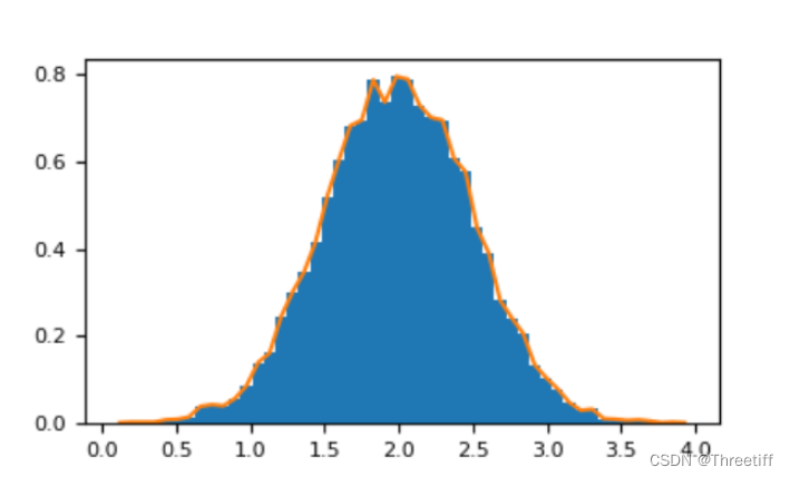
# Build a vector of 10000 normal deviates with variance 0.5^2 and mean 2
mu, sigma = 2, 0.5
v = rg.normal(mu, sigma, 10000)
# Plot a normalized histogram with 50 bins
plt.hist(v, bins=50, density=True) # matplotlib version (plot)
(array...)
# Compute the histogram with numpy and then plot it
(n, bins) = np.histogram(v, bins=50, density=True) # NumPy version (no plot)
plt.plot(.5 * (bins[1:] + bins[:-1]), n) # bins[1:]指从第一个数据到最后一个数据,bins[:-1]指从第0个数据到倒数第二个数据,前后两个bin的值求平均
参考链接: