数据可视化01_t-SNE

1. t-SNE的定义

t-SNE stands for t-distributed Stochastic Neighbor Embedding.
代表 t 分布随机邻域嵌入。

t-SNE 获取高维数据并将其降低到较低维空间，同时保持数据点之间的关系尽可能接近其原始排列。

它是一种无监督机器学习算法，由 Laurens van der Maaten 和 Geoffery Hinton 于 2008 年开发。

这就是 t-SNE 的工作原理，步骤很简单：

1.1. 测量高维空间中的相似性

1. 首先，t-SNE 测量原始高维空间中数据点之间的相似性。
2. 它计算点之间的成对距离，并使用高斯分布将其转换为概率。
3. 概率表示两个点彼此相邻的可能性。

1.2表示低维空间中的相似性

1. 接下来，t-SNE 创建一个低维空间（2D 或 3D）并初始化每个数据点的随机坐标。
2. 然后，它计算低维空间中这些点之间的成对距离，并使用 t 分布将它们转换为概率。

1.3 优化

目标是使低维空间中的概率与高维空间中的概率相似。

这是通过梯度下降来最小化称为 Kullback-Leibler (KL) 散度的成本函数来完成的，该函数衡量两个概率分布之间的差异。

1.4 t-SNE 与主成分分析 (PCA) 有何不同？

t-SNE 是一种非线性降维算法，与 PCA（一种线性降维算法）不同。

虽然主成分分析 (PCA) 假设数据具有线性关系，但 t-SNE 并不这样假设。

因此，t-SNE 在现实世界非线性数据的降维方面更有用。

2. 各类任务举例

2.1　t-SNE on Iris Dataset Iris

鸢尾花数据集包含来自三个不同物种的 150 个鸢尾花样本：山鸢尾、杂色鸢尾和维吉尼亚鸢尾。

每个样本都有四个特征： sepal length 、 sepal width 、 petal length 和 petal width 。

让我们可视化在此数据集上应用 t-SNE 后获得的结果，它将 4 维表示转换为 2 维表示。

import numpy as np
import matplotlib.pyplot as plt
from sklearn.datasets import load_iris
from sklearn.manifold import TSNE

# Load the Iris dataset
iris = load_iris()
X, y = iris.data, iris.target

# Perform t-SNE
tsne = TSNE(n_components=2, perplexity=30, random_state=42)
X_tsne = tsne.fit_transform(X)

# Visualize the results
plt.figure(figsize=(8, 6))
scatter = plt.scatter(X_tsne[:, 0], X_tsne[:, 1], c=y, cmap="viridis", alpha=0.8)

cbar = plt.colorbar(scatter, ticks=range(3))
cbar.ax.set_yticklabels(['Iris setosa', 'Iris versicolor', 'Iris virginica']) 

plt.title("Iris Dataset t-SNE Visualization")
plt.xlabel("t-SNE 1st Component")
plt.ylabel("t-SNE 2nd Component")
plt.show()

Perplexity? 什么是困惑度？

perplexity 是与 t-SNE 一起使用的超参数，用于确定在高维空间中构建概率分布时为每个数据点考虑的邻居数量。

当 t-SNE 应用于鸢尾花数据集时，生成的图显示了对应于三种鸢尾花物种的三个不同簇。

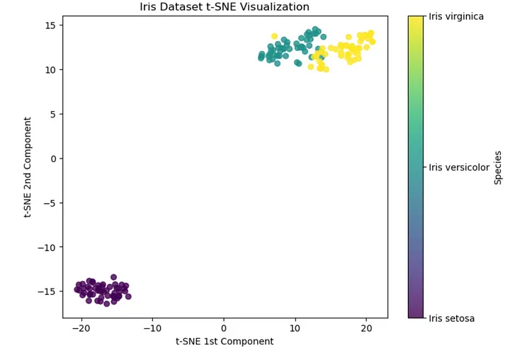
请注意，Iris versicolor 和 Iris virginica 的成分重叠，表明这些物种有更多相似之处。

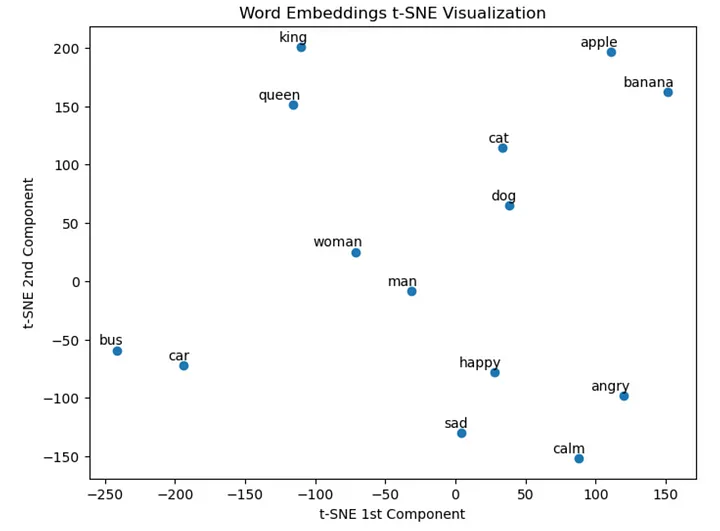
2.2　t-SNE on GloVe Embeddings

GloVe (Global Vectors for Word Representation)，

GloVe（单词表示的全局向量）是一种无监督学习算法，用于获取单词的向量表示（也称为嵌入）。

请注意，这些嵌入是多维的，我们将在二维空间中使用 t-SNE。

import numpy as np
import matplotlib.pyplot as plt
from sklearn.manifold import TSNE
from gensim.downloader import load

# Load the pre-trained GloVe word embeddings
glove_vectors = load("glove-wiki-gigaword-50")

# Select a subset of words to visualize
words_to_visualize = ["king", "queen", "man", "woman", "dog", "cat", "car", "bus", "apple", "banana", "happy", "sad", "angry", "calm"]

# Get the corresponding word vectors
word_vectors = np.array([glove_vectors[word] for word in words_to_visualize])

# Perform t-SNE
tsne = TSNE(n_components=2, perplexity=5, random_state=42)
word_vectors_tsne = tsne.fit_transform(word_vectors)

# Visualize the results
plt.figure(figsize=(8, 6))
scatter = plt.scatter(word_vectors_tsne[:, 0], word_vectors_tsne[:, 1])

# Add labels to the points
for i, word in enumerate(words_to_visualize):
    plt.annotate(word, xy=(word_vectors_tsne[i, 0], word_vectors_tsne[i, 1]), xytext=(5, 2), textcoords="offset points", ha="right", va="bottom")

plt.title("Word Embeddings t-SNE Visualization")
plt.xlabel("t-SNE 1st Component")
plt.ylabel("t-SNE 2nd Component")

plt.show()

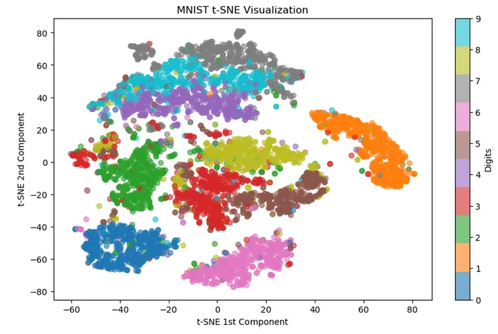
2.3　t-SNE on MNIST Dataset MNIST

MNIST 数据集由 70,000 个从 0 到 9 的手写数字组成，每个数字表示为 28x28 像素的灰度图像。

每个图像都表示为 784 维向量 ( 28 * 28 = 784 )。

让我们在二维空间中可视化这些图像。

import numpy as np
import matplotlib.pyplot as plt
from sklearn.datasets import fetch_openml
from sklearn.decomposition import PCA
from sklearn.manifold import TSNE
from sklearn.model_selection import train_test_split
from sklearn.preprocessing import StandardScaler

# Load the MNIST dataset
mnist = fetch_openml("mnist_784")
X, y = mnist.data, mnist.target

请注意，我们将首先使用 StandardScaler 缩放数据，然后选择 5000 个图像的子集以加快计算速度。

# Preprocess the data
scaler = StandardScaler()
X_scaled = scaler.fit_transform(X)

# Select a subset of the dataset for faster computation
X_subset, _, y_subset, _ = train_test_split(X_scaled, y, train_size=5000, random_state=42, stratify=y)

t-SNE 的 sklearn 文档告诉我们，如果特征数量非常多，强烈建议使用另一种降维方法（例如 PCA）将维度数减少到合理的数量（例如 50）。高（在我们的例子中为 784）。

因此，在应用 t-SNE 之前，我们将使用 PCA 将 MNIST 数据集的维度从 784 维降低到 50 维。

# Perform PCA for faster t-SNE computation
pca = PCA(n_components=50)
X_pca = pca.fit_transform(X_subset)

接下来，让我们执行 t-SNE 并可视化结果。

# Perform t-SNE
tsne = TSNE(n_components=2, perplexity=30, random_state=42)
X_tsne = tsne.fit_transform(X_pca)

# Visualize the results
plt.figure(figsize=(12, 8))
scatter = plt.scatter(X_tsne[:, 0], X_tsne[:, 1], c=y_subset.astype(int), cmap="tab10", alpha=0.6)
plt.colorbar(scatter, ticks=range(10), label="Digits")
plt.title("MNIST t-SNE Visualization")
plt.xlabel("t-SNE 1st Component")
plt.ylabel("t-SNE 2nd Component")
plt.show()