首先我事先准备好五分类的图片放在对应的文件夹,图片资源在我的gitee文件夹中链接如下:文件管理: 用于存各种数据https://gitee.com/xiaoxiaotai/file-management.git
里面有imgs目录和npy目录,imgs就是存放5分类的图片的目录,里面有桂花、枫叶、五味子、银杏、竹叶5种植物,npy目录存放的是我用这些图片制作好的npy文件数据集,里面有32x32大小和64x64大小的npy文件。
接下来是数据集制作过程:
首先导入所需的库
import os
import cv2
import random
import numpy as np
import matplotlib.pyplot as plt
import matplotlib.image as mpimg
from mpl_toolkits.axes_grid1 import ImageGrid
%matplotlib inline
import math
from tqdm import tqdm
下面是先显示本地分类中部分图片
#先显示枫叶图片
folder_path = './datas/imgs/fengye'
# 可视化图像的个数
N = 36
# n 行 n 列
n = math.floor(np.sqrt(N))

images = []
for each_img in os.listdir(folder_path)[:N]:
    img_path = os.path.join(folder_path, each_img)
    #img_bgr = cv2.imread(img_path)
    img_bgr = cv2.imdecode(np.fromfile(img_path, dtype=np.uint8), 1) #解决路径中存在中文的问题
    img_rgb = cv2.cvtColor(img_bgr, cv2.COLOR_BGR2RGB)
    images.append(img_rgb)

fig = plt.figure(figsize=(6, 8),dpi=80)
grid = ImageGrid(fig, 111,  # 类似绘制子图 subplot(111)
                 nrows_ncols=(n, n),  # 创建 n 行 m 列的 axes 网格
                 axes_pad=0.02,  # 网格间距
                 share_all=True
                 )

# 遍历每张图像
for ax, im in zip(grid, images):
    ax.imshow(im)
    ax.axis('off')

plt.tight_layout()
plt.show()
输出结果如下:

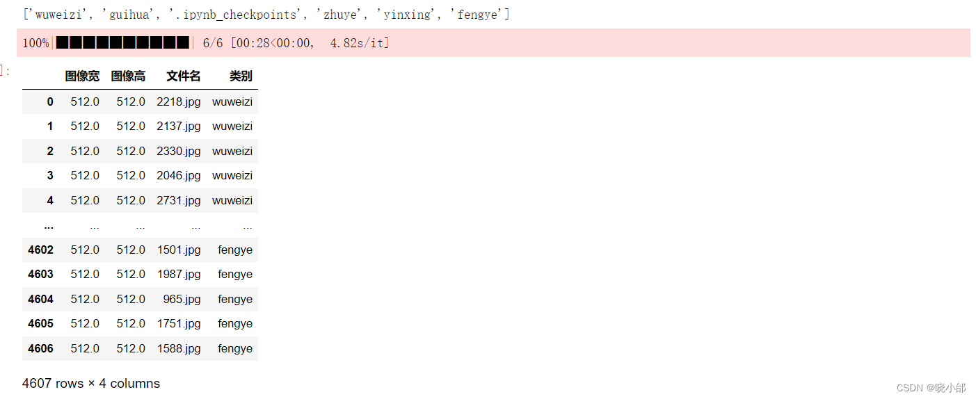
下面是输出各个图片的信息包括图片宽高、图片名、所属类别,os.chdir('../')意思是将当前路径指针指向上一个目录,可以用os.getcwd()输出当前所指路径
# 指定数据集路径
dataset_path = './datas/imgs/'
os.chdir(dataset_path)
print(os.listdir())

df = pd.DataFrame()
for fruit in tqdm(os.listdir()): # 遍历每个类别
    os.chdir(fruit)
    for file in os.listdir(): # 遍历每张图像
        try:
            img = cv2.imread(file)
            df = df.append({'类别':fruit, '文件名':file, '图像宽':img.shape[1], '图像高':img.shape[0]}, ignore_index=True)
        except:
            print(os.path.join(fruit, file), '读取错误')
    os.chdir('../')
os.chdir('../../')
df
输出结果如下:
定义标签数字,因为数据集标签一般是数字,训练才更快
# 定义5个类别的标签
labels = {
    'wuweizi': 0,
    'fengye': 1,
    'guihua': 2,
    'zhuye': 3,
    'yinxing': 4
}

# 定义训练集和测试集的比例
train_ratio = 0.8

# 定义一个空列表用于存储训练集和测试集
train_data = []
test_data = []
数据增强,我这里是将每一张图片缩小为64x64,你也可以改成32x32或者其他大小,要注意的是,大小越大数据集制作越久,得到的数据集大小越大。
# 定义数据增强的方法
def data_augmentation(img):
    # 随机裁剪
    img = cv2.resize(img, (256, 256))
    x = random.randint(0, 256 - 64)
    y = random.randint(0, 256 - 64)
    img = img[x:x+64, y:y+64]


    # 随机翻转
    if random.random() < 0.5:
        img = cv2.flip(img, 1)

    # 随机旋转
    angle = random.randint(-10, 10)
    M = cv2.getRotationMatrix2D((32, 32), angle, 1)
    img = cv2.warpAffine(img, M, (64, 64))

    return img
# 定义读取图片的方法
def read_image(path):
img = cv2.imread(path)
img = cv2.cvtColor(img, cv2.COLOR_BGR2RGB)
img = data_augmentation(img)
img = img / 255.0
return img下面是给图片打上标签了,也就是每一张图片都给它标注属于哪一种类别(身份),这样卷积神经网络就可以在训练的时候知道类别,从而记住所属特征的标签值
# 遍历5个文件夹,读取图片并打上标签
for path, label in labels.items():
files = os.listdir('./datas/imgs/'+path)
random.shuffle(files)
train_files = files[:int(len(files) * train_ratio)]
test_files = files[int(len(files) * train_ratio):]
for file in train_files:
img = read_image(os.path.join('./datas/imgs/'+path, file))
train_data.append((img, label))
for file in test_files:
img = read_image(os.path.join('./datas/imgs/'+path, file))
test_data.append((img, label))
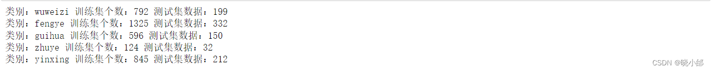
# 工整地输出每一类别的数据个数
print('类别:{} 训练集个数:{} 测试集数据:{}'.format(path, len(train_files), len(test_files)))这里的输出结果:
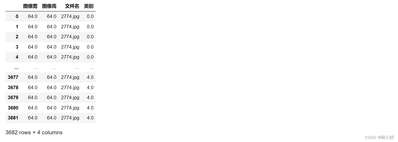
现在可以看一下裁剪后的结果
df = pd.DataFrame()
for img,label in train_data: # 遍历每个类别

#     img = cv2.imread(fruit)
    df = df.append({'类别':label, '文件名':file, '图像宽':img.shape[1], '图像高':img.shape[0]}, ignore_index=True)
df
结果如下,我们可以看到大小已经变成64x64了,当然这是没有打乱顺序的,类别是从0开始到4:
接下来就是打乱顺序,这也是为了防止过拟合化
# 打乱训练集和测试集的顺序
random.shuffle(train_data)
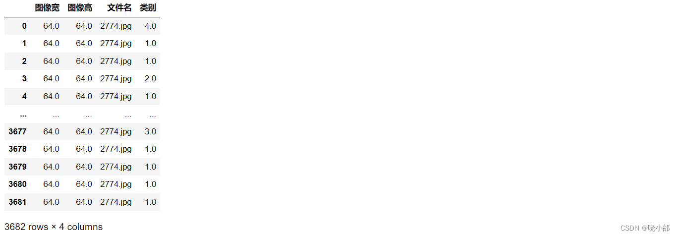
random.shuffle(test_data)再次输出
df = pd.DataFrame()
for img,label in train_data: # 遍历每个类别

#     img = cv2.imread(fruit)
    df = df.append({'类别':label, '文件名':file, '图像宽':img.shape[1], '图像高':img.shape[0]}, ignore_index=True)
df
这一次的结果如下,类别顺序已经被打乱:
下面是保存训练集和测试集的数据集和标签
# 将训练集和测试集的图片和标签分别存储在numpy数组中
train_imgs = np.array([data[0] for data in train_data])
train_labels = np.array([data[1] for data in train_data])
test_imgs = np.array([data[0] for data in test_data])
test_labels = np.array([data[1] for data in test_data])

# 保存训练集和测试集
np.save('./datas/npy/32px/train_imgs_64.npy', train_imgs)
np.save('./datas/npy/32px/train_labels_64.npy', train_labels)
np.save('./datas/npy/32px/test_imgs_64.npy', test_imgs)
np.save('./datas/npy/32px/test_labels_64.npy', test_labels)
上面的数据集已经做好了,那么接下来就到模型的训练了,模型的训练我就不一一解释了,大家自己看代码,我使用的是anaconda中的jupyter工具写代码
#导库
import tensorflow as tf
import numpy as np
import os
import matplotlib.pyplot as plt
import urllib
import cv2

# 加载上面制作的数据集
train_imgs = np.load('./datas/npy/64px/train_imgs_64.npy')
train_labels = np.load('./datas/npy/64px/train_labels_64.npy')
test_imgs = np.load('./datas/npy/64px/test_imgs_64.npy')
test_labels = np.load('./datas/npy/64px/test_labels_64.npy')

#可以看看输出纬度
train_imgs.shape

#模型构建,这里我就构建一个简单模型
def creatAlexNet():
    model = tf.keras.models.Sequential([
        tf.keras.layers.Conv2D(64, kernel_size=(3, 3), strides=(1, 1), activation='relu', input_shape=(64, 64, 3)),
        tf.keras.layers.MaxPooling2D(pool_size=(2, 2), strides=(1, 1)),
        tf.keras.layers.Conv2D(128, kernel_size=(3, 3), strides=(1, 1), activation='relu'),
        tf.keras.layers.MaxPooling2D(pool_size=(2, 2), strides=(1, 1)),
        tf.keras.layers.Flatten(),
        tf.keras.layers.Dense(5, activation='softmax')
    ])
    return model

#加载模型
model = creatAlexNet()

#显示摘要
model.summary()


# 定义超参数
learning_rate = 0.001 #study
batch_size = 100 #单次训练样本数(批次大小)
epochs = 20 #训练轮数

# 定义训练模式
model.compile(optimizer ='adam',#优化器
loss='sparse_categorical_crossentropy',#损失函数
              metrics=['accuracy'])#评估模型的方式

# 加载数据集并训练模型
history = model.fit(train_imgs, train_labels, batch_size=batch_size, epochs=epochs,
                    validation_split = 0.2)

# 评估模型
test_loss, test_acc = model.evaluate(test_imgs, test_labels, verbose=2)
print('Test accuracy:', test_acc)

#模型测试
preds = model.predict(test_imgs)
np.argmax(preds[20])

# 可视化测试
# 定义显示图像数据及其对应标签的函数
# 图像列表
label_dict={0:"wuweizi",1:"fengye",2:"guihua",3:"zhuye",4:"yinxing"}
def plot_images_labels_prediction(images,# 标签列表
                                  labels,
                                  preds,#预测值列表
                                  index,#从第index个开始显示
                                  num = 5):  # 缺省一次显示5幅
    fig=plt.gcf()#获取当前图表,Get Current Figure
    fig.set_size_inches(12,6)#1英寸等于2.54cm
    if num > 10:#最多显示10个子图
        num = 10
    for i in range(0, num):
        ax = plt.subplot(2,5,i+1)#获取当前要处理的子图
        plt.tight_layout()
        ax.imshow(images[index])
        title=str(i)+','+label_dict[labels[index]]#构建该图上要显示的title信息
        if len(preds)>0:
            title +='=>' + label_dict[np.argmax(preds[index])]
        ax.set_title(title,fontsize=10)#显示图上的title信息
        index += 1
    plt.show()

plot_images_labels_prediction(test_imgs,test_labels, preds,10,30)

# 然后保存模型
model_filename ='models/plant_model.h5'
model.save(model_filename)

# 这里是从本地加载图片对模型进行测试
from PIL import Image
import numpy as np

loaded_model = tf.keras.models.load_model('models/plant_model.h5')
label_dict={0:"wuweizi",1:"fengye",2:"guihua",3:"zhuye",4:"yinxing"}

img = Image.open('./fengye.jpeg')
img = img.resize((64, 64))
img_arr = np.array(img) / 255.0
img_arr = img_arr.reshape(1, 64, 64, 3)
pred = model.predict(img_arr)
class_idx = np.argmax(pred)
plt.title("type:{}, pre_label:{}".format(label_dict[class_idx],class_idx))
plt.imshow(img, cmap=plt.get_cmap('gray'))

# 加载模型
loaded_model = tf.keras.models.load_model('models/plant_model.h5')
# 使用模型预测浏览器上的一张图片
label_dict={0:"wuweizi",1:"fengye",2:"guihua",3:"zhuye",4:"yinxing"}

# 这里是从浏览器的网址中加载图片进行识别
url = 'https://newbbs-fd.zol-img.com.cn/t_s1200x5000/g5/M00/05/08/ChMkJ1wFsOGIcMt4AAGFQDPiUhEAAtkTQCj_EoAAYVY306.jpg'
with urllib.request.urlopen(url) as url_response:
    img_array = np.asarray(bytearray(url_response.read()), dtype=np.uint8)
    img = cv2.imdecode(img_array, cv2.IMREAD_COLOR)
    img_array = cv2.resize(img, (64, 64))
    img_array = img_array / 255.0
    img_array = np.expand_dims(img_array, axis=0)

    predict_label = np.argmax(loaded_model.predict(img_array), axis=-1)[0]
    plt.imshow(img, cmap=plt.get_cmap('gray'))
    plt.title("Predict: {},Predict_label: {}".format(label_dict[predict_label],predict_label))
    plt.xticks([])
    plt.yticks([])
本次文章就到这里,感谢大家的支持!