以下都是建模常用模型的代码,都是纯代码(可能有点多),如果对模型理论还不熟悉的同学,建议先过一下理论,这样能更好的理解和实践代码。国赛快开始了,让我们一起来玩转这些模型的代码吧。
常规优化模型
优化问题在数学建模比赛中十分常见,熟练掌握如何使用一些常用的优化模型可以大大的加快我们在比赛中解题的速度。常规的优化模型有: 线性规划,非线性规划,整数规划,整数规划, 多目标规划,动态规划。
线性规划
m i n z = 2 x 1 + 3 x 2 + x 3 min z = 2x_1+3x_2 +x_3 minz=2x1+3x2+x3
s t . { x 1 + 4 x 2 + 2 x 3 ≥ 8 3 x 1 + 2 x 2 ≥ 6 x 1 , x 2 , x 3 ≥ 0 st. \begin{cases} x_1+4x_2 +2x_3\geq8 \\ 3x_1+2x_2 \geq6\\ x_1,x_2,x_3\geq0\\ \end{cases} st.⎩⎪⎨⎪⎧x1+4x2+2x3≥83x1+2x2≥6x1,x2,x3≥0
import numpy as np
from scipy.optimize import linprog

c = np.array([2, 3, 1])
A_up = np.array([[-1, -4, -2], [-3, -2, 0]])
b_up = np.array([-8, -6])
r = linprog(c, A_ub=A_up, b_ub=b_up, bounds=((0, None), (0, None), (0, None)))
print(r)
非线性规划
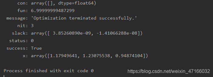
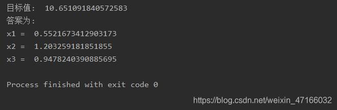
m i n f ( x ) = x 1 2 + x 2 2 + x 3 2 + 8 min f(x) = x_1^2+x_2^2 +x_3^2+8 minf(x)=x12+x22+x32+8
s t . { x 1 3 − x 2 + x 3 2 ≥ 0 x 1 + x 2 2 + x 3 2 ≤ 20 − x 1 − x 2 2 + 2 = 0 x 2 + 2 x 3 2 = 3 x 1 , x 2 , x 3 > 0 st. \begin{cases} x_1^3-x_2 +x_3^2\geq0 \\ x_1+x_2^2+x_3^2\leq20\\ -x_1-x_2^2+2=0\\ x_2+2x_3^2=3\\ x_1,x_2,x_3>0\\ \end{cases} st.⎩⎪⎪⎪⎪⎪⎪⎨⎪⎪⎪⎪⎪⎪⎧x13−x2+x32≥0x1+x22+x32≤20−x1−x22+2=0x2+2x32=3x1,x2,x3>0
import numpy as np
from scipy.optimize import minimize

# 边界约束
b = (0.0, None)
bnds = (b, b, b)
f = lambda x: x[0] ** 2 + x[1] **2 + x[2] ** 2 + 8
cons = ({

    'type': 'ineq', 'fun': lambda x: x[0]**2 - x[1] + x[2]**2},
        {

    'type': 'ineq', 'fun': lambda x: -x[0] - x[1] - x[2]**3 + 20},
        {

    'type': 'eq', 'fun': lambda x: -x[0] - x[1]**2 + 2},
        {

    'type': 'eq', 'fun': lambda x: x[1] + 2 * x[2]**2 - 3})  # 4个约束条件,eq是=; ineq是>=
x0 = np.array([0, 0, 0])
# 计算
solution = minimize(f, x0, method='SLSQP',  bounds=bnds, constraints=cons)
x = solution.x
print('目标值: ', str(f(x)))
print('答案为:')
print('x1 = ', str(x[0]))
print('x2 = ', str(x[1]))
print('x3 = ', str(x[2]))
整数规划
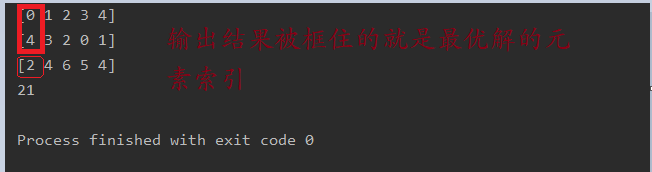
匈牙利算法
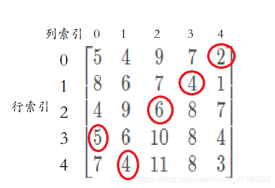
矩阵
[ 5 4 9 7 2 8 6 7 4 1 4 9 6 8 7 5 6 10 8 4 7 4 11 8 3 ] \left[ \begin{matrix} 5 &4&9& 7& 2 \\ 8& 6& 7& 4& 1 \\ 4&9& 6&8&7 \\ 5&6&10& 8& 4\\ 7&4&11& 8& 3\\ \end{matrix} \right] ⎣⎢⎢⎢⎢⎡584574696497610117488821743⎦⎥⎥⎥⎥⎤
import numpy as np
from scipy.optimize import linear_sum_assignment

cost = np.array([[5, 4, 9, 7, 2], [8, 6, 7, 4, 1], [4, 9, 6, 8, 7], [5, 6, 10, 8, 4], [7, 4, 11, 8, 3]])
row_index, column_index = linear_sum_assignment(cost)
print(row_index)  # 行索引
print(column_index)  # 行索引的最优指派的列索引
print(cost[row_index, column_index])  # 每个行索引的最优指派列索引所在的元素
print(cost[row_index, column_index].sum())  # 求和
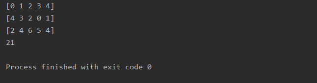
输出结果理解:
蒙特卡罗算法
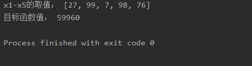
max z = x 1 2 + x 2 2 + 3 x 3 2 + 4 x 4 2 + 2 x 5 2 − 8 x 1 − 2 x 2 − 3 x 3 − x 4 − 2 x 5 \max z = x_1^2+x_2^2 +3x_3^2+4x_4^2+2x_5^2-8x_1-2x_2-3x_3-x_4-2x_5 maxz=x12+x22+3x32+4x42+2x52−8x1−2x2−3x3−x4−2x5
s t . { 0 ≤ x i ≤ 99 , i = 1 , 2 , 3... , 5 , x 1 + x 2 + x 3 + x 4 + x 5 ≤ 400 , x 1 + 2 x 2 + 2 x 3 + x 4 + 6 x 5 ≤ 800 , 2 x 1 + x 2 + 6 x 3 ≤ 200 , x 3 + x 4 + 5 x 5 ≤ 500 st. \begin{cases} 0\leq x_i\leq 99,i=1,2,3...,5, \\ x_1+x_2+x_3+x_4+x_5\leq400,\\ x_1+2x_2+2x_3+x_4+6x_5\leq800,\\ 2x_1+x_2+6x_3\leq200,\\ x_3+x_4+5x_5\leq500\\ \end{cases} st.⎩⎪⎪⎪⎪⎪⎪⎨⎪⎪⎪⎪⎪⎪⎧0≤xi≤99,i=1,2,3...,5,x1+x2+x3+x4+x5≤400,x1+2x2+2x3+x4+6x5≤800,2x1+x2+6x3≤200,x3+x4+5x5≤500
import time
import random


# 目标函数
def f(x: list) -> int:
    return x[0] ** 2 + x[1] ** 2 + 3 * x[2] ** 2 + 4 * x[3] ** 2 + 2 * x[4] ** 2 - 8 * x[0] - 2 * x[1] - 3 * x[2] - x[
        3] - 2 * x[4]


# 约束向量函数
def g(x: list) -> list:
    res=[]
    res.append(sum(x) - 400)
    res.append(x[0] + 2 * x[1] + 2 * x[2] + x[3] + 6 * x[4] - 800)
    res.append(2 * x[0] + x[1] + 6 * x[2] - 200)
    res.append(x[2] + x[3] + 5 * x[4] - 500)
    return res


random.seed(time.time)
pb = 0
xb = []
for i in range(10 ** 6):
    x = [random.randint(0, 99) for i in range(5)]  # 产生一行五列的区间[0, 99] 上的随机整数
    rf = f(x)
    rg = g(x)
    if all((a < 0 for a in rg)):  # 若 rg 中所有元素都小于 0
        if pb < rf:
            xb = x
            pb = rf
print('x1-x5的取值:', xb)
print('目标函数值:', pb)
由于蒙特卡罗算法是随机模拟,所以最后的答案都是不同的
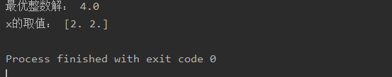
分支定界法(python实现)
max z = x 1 + x 2 \max z = x_1+x_2 maxz=x1+x2
s t . { 14 x 1 + 9 x 2 ≤ 51 − 6 x 1 + 3 x 2 ≤ 1 x 1 , x 2 ≥ 0 x 1 , x 2 且 为 整 数 st. \begin{cases} 14x_1+9x_2 \leq51 \\ -6x_1+3x_2\leq1\\ x_1,x_2\geq0 \\ x_1,x_2且为整数 \end{cases} st.⎩⎪⎪⎪⎨⎪⎪⎪⎧14x1+9x2≤51−6x1+3x2≤1x1,x2≥0x1,x2且为整数
from scipy.optimize import linprog
import numpy as np
import math
import sys
from queue import Queue


class ILP():
    def __init__(self, c, A_ub, b_ub, A_eq, b_eq, bounds):
        # 全局参数
        self.LOWER_BOUND=-sys.maxsize
        self.UPPER_BOUND=sys.maxsize
        self.opt_val=None
        self.opt_x=None
        self.Q=Queue()

        # 这些参数在每轮计算中都不会改变
        self.c=-c
        self.A_eq=A_eq
        self.b_eq=b_eq
        self.bounds=bounds

        # 首先计算一下初始问题
        r=linprog(-c, A_ub, b_ub, A_eq, b_eq, bounds)

        # 若最初问题线性不可解
        if not r.success:
            raise ValueError('Not a feasible problem!')

        # 将解和约束参数放入队列
        self.Q.put((r, A_ub, b_ub))

    def solve(self):
        while not self.Q.empty():
            # 取出当前问题
            res, A_ub, b_ub=self.Q.get(block=False)

            # 当前最优值小于总下界,则排除此区域
            if -res.fun < self.LOWER_BOUND:
                continue

            # 若结果 x 中全为整数,则尝试更新全局下界、全局最优值和最优解
            if all(list(map(lambda f: f.is_integer(), res.x))):
                if self.LOWER_BOUND < -res.fun:
                    self.LOWER_BOUND=-res.fun

                if self.opt_val is None or self.opt_val < -res.fun:
                    self.opt_val=-res.fun
                    self.opt_x=res.x

                continue

            # 进行分枝
            else:
                # 寻找 x 中第一个不是整数的,取其下标 idx
                idx=0
                for i, x in enumerate(res.x):
                    if not x.is_integer():
                        break
                    idx+=1

                # 构建新的约束条件(分割
                new_con1=np.zeros(A_ub.shape[1])
                new_con1[idx]=-1
                new_con2=np.zeros(A_ub.shape[1])
                new_con2[idx]=1
                new_A_ub1=np.insert(A_ub, A_ub.shape[0], new_con1, axis=0)
                new_A_ub2=np.insert(A_ub, A_ub.shape[0], new_con2, axis=0)
                new_b_ub1=np.insert(
                    b_ub, b_ub.shape[0], -math.ceil(res.x[idx]), axis=0)
                new_b_ub2=np.insert(
                    b_ub, b_ub.shape[0], math.floor(res.x[idx]), axis=0)

                # 将新约束条件加入队列,先加最优值大的那一支
                r1=linprog(self.c, new_A_ub1, new_b_ub1, self.A_eq,
                           self.b_eq, self.bounds)
                r2=linprog(self.c, new_A_ub2, new_b_ub2, self.A_eq,
                           self.b_eq, self.bounds)
                if not r1.success and r2.success:
                    self.Q.put((r2, new_A_ub2, new_b_ub2))
                elif not r2.success and r1.success:
                    self.Q.put((r1, new_A_ub1, new_b_ub1))
                elif r1.success and r2.success:
                    if -r1.fun > -r2.fun:
                        self.Q.put((r1, new_A_ub1, new_b_ub1))
                        self.Q.put((r2, new_A_ub2, new_b_ub2))
                    else:
                        self.Q.put((r2, new_A_ub2, new_b_ub2))
                        self.Q.put((r1, new_A_ub1, new_b_ub1))


def input_function():
    c = np.array([1, 1])
    A_ub = np.array([[14, 9], [-6, 3]])
    b_ub = np.array([51, 1])
    Aeq = None
    beq = None
    bounds = [(0, None), (0, None)]
    solver = ILP(c, A_ub, b_ub, Aeq, beq, bounds)
    solver.solve()
    print("最优整数解:", solver.opt_val)
    print("x的取值:", solver.opt_x)


if __name__ == '__main__':
    input_function()
多目标规划
多目标规划其实最后可以转为单目标规划,下面有两种多目标规划方法和对应代码
方法一:最大化一个目标,然后将其添加为约束并解决另一个目标
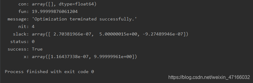
max z 1 = 2 x 1 + 3 x 2 \max z_1 = 2x_1+3x_2 maxz1=2x1+3x2
max z 2 = 4 x 1 − 2 x 2 \max z_2=4x_1-2x_2 maxz2=4x1−2x2
s t . { x 1 + x 2 ≤ 10 2 x 1 + x 2 ≤ 15 x 1 , x 2 ≥ 0 x 1 , x 2 ∈ R st. \begin{cases} x_1+x_2 \leq10 \\ 2x_1+x_2\leq15\\ x_1,x_2\geq0 \\ x_1,x_2\in R\\ \end{cases} st.⎩⎪⎪⎪⎨⎪⎪⎪⎧x1+x2≤102x1+x2≤15x1,x2≥0x1,x2∈R
import numpy as np
from scipy.optimize import linprog


def max_target():
    f = lambda x: 2*x[0] + 3*x[1]  # 第一个要优化的函数
    c = np.array([-2, -3])
    A_up = np.array([[1, 1], [2, 1]])
    b_up = np.array([10, 15])
    r = linprog(c, A_ub=A_up, b_ub=b_up, bounds=((0, None), (0, None)))  # 进行线性优化,如果是非线性,选择非线性模型
    return f(r.x)


def max_end():
    f_1 = lambda x: 4 * x[0] - 2 * x[1]  # 最后要优化的函数
    c = np.array([-4, 2])
    A_up = np.array([[1, 1], [2, 1], [-2, -3]])
    b_up = np.array([10, 15, -max_target()])
    r = linprog(c, A_ub=A_up, b_ub=b_up, bounds=((0, None), (0, None)))  # 把第一个函数当作约束项,并且大于等于它的最优解
    print(r)


if __name__ == '__main__':
    max_target()
    max_end()
方法二:使用采样的权重和具有定义步长的迭代组合目标
max z = a ( 2 x 1 + 3 x 2 ) + ( 1 − a ) 4 x 1 − 2 x 2 \max z =a(2x_1+3x_2)+(1-a)4x_1-2x_2 maxz=a(2x1+3x2)+(1−a)4x1−2x2
s t . { x 1 + x 2 ≤ 10 2 x 1 + x 2 ≤ 15 x 1 , x 2 ≥ 0 x 1 , x 2 ∈ R st. \begin{cases} x_1+x_2 \leq10 \\ 2x_1+x_2\leq15\\ x_1,x_2\geq0 \\ x_1,x_2\in R\\ \end{cases} st.⎩⎪⎪⎪⎨⎪⎪⎪⎧x1+x2≤102x1+x2≤15x1,x2≥0x1,x2∈R
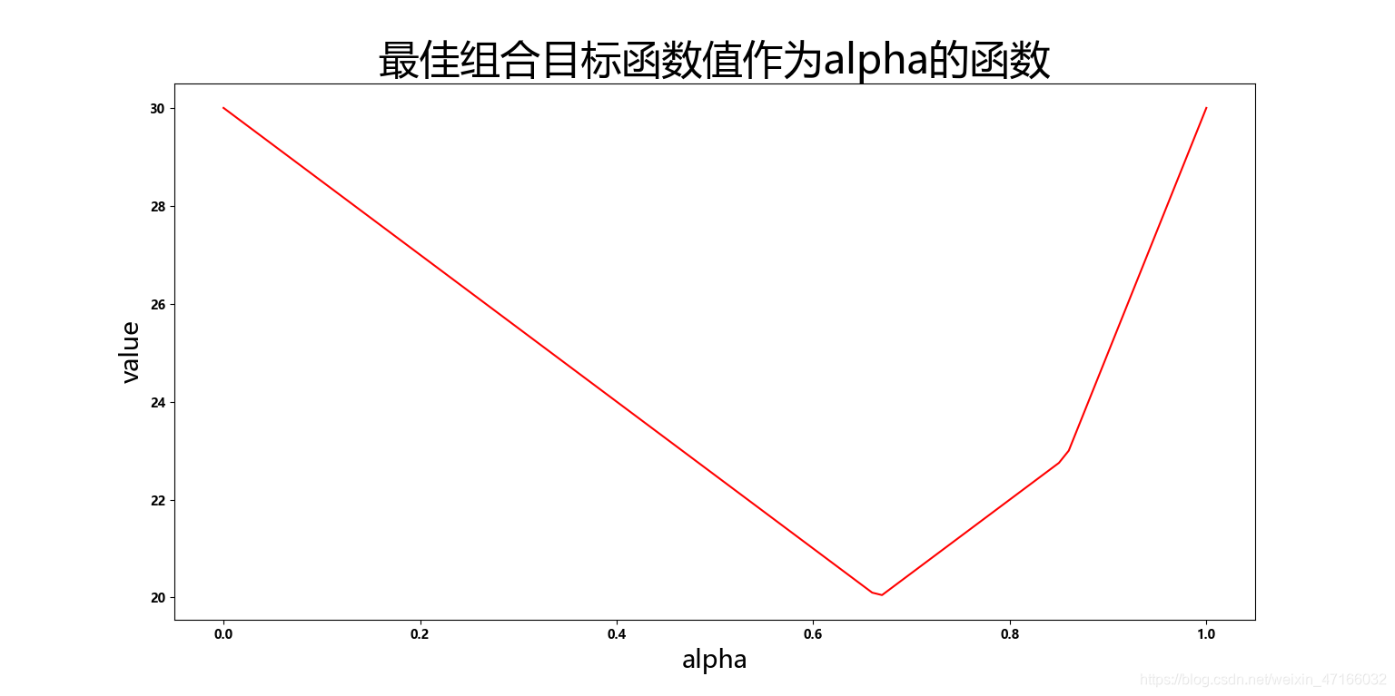
现在多目标规划变单目标只有解决如何选取a就可以了。在这种情况下,典型的方法是确定有效边界。在经济学中,例如被称为“最佳最优”。为了构建这样的方法,我以0.01的步长采样alpha。对于每个alpha值,使用PuLP重新说明问题,然后加以解决。
import matplotlib.pyplot as plt
import numpy as np
import pandas as pd
import pulp
# 定义步长
stepSize = 0.01
# 使用PuLP的delcare优化变量
x1 = pulp.LpVariable("x1", lowBound=0)
x2 = pulp.LpVariable("x2", lowBound=0)
# 初始化空的DataFrame以存储优化结果
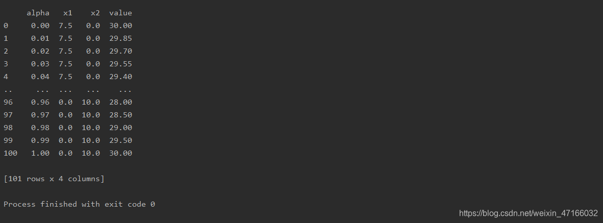
solutionTable = pd.DataFrame(columns=["alpha", "x1", "x2", "value"])
# 使用stepSize迭代从0到1的alpha值,并将pulp算出的结果写入solutionTable
for i in range(0, 101, int(stepSize*100)):
linearProblem = pulp.LpProblem(" 多目标线性最大化 ", pulp.LpMaximize) # 声明函数
linearProblem += (i/100)*(2*x1+3*x2)+(1-i/100)*(4*x1-2*x2) # 在采样的alpha处添加目标函数
linearProblem += x1 + x2 <= 10
linearProblem += 2*x1 + x2 <= 15 # 添加约束
solution = linearProblem.solve() # 得出解
solutionTable.loc[int(i/(stepSize*100))] = [i/100, pulp.value(x1), pulp.value(x2),
pulp.value(linearProblem.objective)] # 将解写入DataFrame
# 使用matplotlib.pyplot可视化优化结果
plt.rc("font", family='MicroSoft YaHei', weight="bold")
plt.figure(figsize=(10, 8))
plt.plot(solutionTable["alpha"], solutionTable["value"], color="red")
plt.xlabel("alpha", size=20)
plt.ylabel("value", size=20)
plt.title(" 最佳组合目标函数值作为alpha的函数 ", size=32)
plt.show()
print(solutionTable)
动态规划
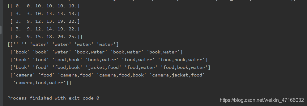
0-1背包问题:现有物品重量和价值1.water[3,10],book[1,3],food[2,9],jacket[2,5],camera[1,6] (前者为重量,后者为价值)。背包最大载重量为6,请问装什么可以使价值最大?
# 动态规划
import numpy as np

# 定义重量
weight = {

    "water": 3, "book": 1, "food": 2, "jacket": 2, "camera": 1}
# 定义价值
worth = {

    "water": 10, "book": 3, "food": 9, "jacket": 5, "camera": 6}
# 存放行标对应的物品名:
table_name = {

    }
table_name[0] = "water"
table_name[1] = "book"
table_name[2] = "food"
table_name[3] = "jacket"
table_name[4] = "camera"
# 创建矩阵,用来保存价值表
table = np.zeros((len(weight), 6))
# 创建矩阵,用来保存每个单元格中的价值是如何得到的(物品名)
table_class = np.zeros((len(weight), 6), dtype=np.dtype((np.str_, 500)))
for i in range(0, len(weight)):
    for j in range(0, 6):
        this_weight = weight[table_name[i]]   # 获取重量
        this_worth=worth[table_name[i]]   # 获得价值
        if(i > 0):  # 获取上一个单元格 (i-1,j)的值
            before_worth = table[i - 1, j]
            temp = 0  # 获取(i-1,j-重量)
            if (this_weight <= j):
                temp = table[i - 1, j - this_weight]
            # (i-1,j-this_weight)+求当前商品价值
            # 判断this_worth能不能用,即重量有没有超标,如果重量超标了是不能加的
            synthesize_worth = 0
            if (this_weight - 1 <= j):
                synthesize_worth = this_worth + temp
            # 与上一个单元格比较,哪个大写入哪个
            if (synthesize_worth > before_worth):
                table[i, j] = synthesize_worth
                if (temp == 0):
                    # 他自己就超过了
                    table_class[i][j] = table_name[i]
                else:
                    # 他自己和(i-1,j-this_weight)
                    table_class[i][j] = table_name[i] + "," + table_class[i - 1][j - this_weight]
            else:
                table[i, j] = before_worth
                table_class[i][j] = table_class[i - 1][j]
        else:
            # 没有(i-1,j)那更没有(i-1,j-重量),就等于当前商品价值,或者重量不够,是0
            if (this_weight - 1 <= j):
                table[i, j] = this_worth
                table_class[i][j] = table_name[i]
print(table)
print(table_class)
常用评价模型
层次分析法
import numpy as np
class AHP:
# 相关信息的传入和准备
def __init__(self, array):
# 记录矩阵相关信息
self.array = array
# 记录矩阵大小
self.n = array.shape[0]
# 初始化RI值,用于一致性检验
self.RI_list = [0, 0, 0.52, 0.89, 1.12, 1.26, 1.36, 1.41, 1.46, 1.49, 1.52, 1.54, 1.56, 1.58,
1.59]
# 矩阵的特征值和特征向量
self.eig_val, self.eig_vector = np.linalg.eig(self.array)
# 矩阵的最大特征值
self.max_eig_val = np.max(self.eig_val)
# 矩阵最大特征值对应的特征向量
self.max_eig_vector = self.eig_vector[:, np.argmax(self.eig_val)].real
# 矩阵的一致性指标CI
self.CI_val = (self.max_eig_val - self.n) / (self.n - 1)
# 矩阵的一致性比例CR
self.CR_val = self.CI_val / (self.RI_list[self.n - 1])
# 一致性判断
def test_consist(self):
# 打印矩阵的一致性指标CI和一致性比例CR
print("判断矩阵的CI值为:" + str(self.CI_val))
print("判断矩阵的CR值为:" + str(self.CR_val))
# 进行一致性检验判断
if self.n == 2: # 当只有两个子因素的情况
print("仅包含两个子因素,不存在一致性问题")
else:
if self.CR_val < 0.1: # CR值小于0.1,可以通过一致性检验
print("判断矩阵的CR值为" + str(self.CR_val) + ",通过一致性检验")
return True
else: # CR值大于0.1, 一致性检验不通过
print("判断矩阵的CR值为" + str(self.CR_val) + "未通过一致性检验")
return False
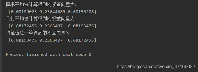
# 算术平均法求权重
def cal_weight_by_arithmetic_method(self):
# 求矩阵的每列的和
col_sum = np.sum(self.array, axis=0)
# 将判断矩阵按照列归一化
array_normed = self.array / col_sum
# 计算权重向量
array_weight = np.sum(array_normed, axis=1) / self.n
# 打印权重向量
print("算术平均法计算得到的权重向量为:\n", array_weight)
# 返回权重向量的值
return array_weight
# 几何平均法求权重
def cal_weight__by_geometric_method(self):
# 求矩阵的每列的积
col_product = np.product(self.array, axis=0)
# 将得到的积向量的每个分量进行开n次方
array_power = np.power(col_product, 1 / self.n)
# 将列向量归一化
array_weight = array_power / np.sum(array_power)
# 打印权重向量
print("几何平均法计算得到的权重向量为:\n", array_weight)
# 返回权重向量的值
return array_weight
# 特征值法求权重
def cal_weight__by_eigenvalue_method(self):
# 将矩阵最大特征值对应的特征向量进行归一化处理就得到了权重
array_weight = self.max_eig_vector / np.sum(self.max_eig_vector)
# 打印权重向量
print("特征值法计算得到的权重向量为:\n", array_weight)
# 返回权重向量的值
return array_weight
if __name__ == "__main__":
# 给出判断矩阵
b = np.array([[1, 1 / 3, 1 / 8], [3, 1, 1 / 3], [8, 3, 1]])
# 算术平均法求权重
weight1 = AHP(b).cal_weight_by_arithmetic_method()
# 几何平均法求权重
weight2 = AHP(b).cal_weight__by_geometric_method()
# 特征值法求权重
weight3 = AHP(b).cal_weight__by_eigenvalue_method()
模糊综合评价
# 模糊综合评价,计算模糊矩阵和指标权重
import xlrd
import math


data = xlrd.open_workbook(r'c:\hufengling\离线数据(更新)\3.xlsx')  # 读取研究数据
# table1 = data.sheets()[0]          # 通过索引顺序获取
# table1 = data.sheet_by_index(sheet_indx)) # 通过索引顺序获取
table2 = data.sheet_by_name('4day')  # 通过名称获取
# rows = table2.row_values(3) # 获取第四行内容
cols1 = table2.col_values(0)  # 获取第1列内容,评价指标1
cols2 = table2.col_values(1)  # 评价指标2
nrow = table2.nrows  # 获取总行数
print(nrow)
# 分为四个等级,优、良、中、差,两个评价指标
u1 = 0
u2 = 0
u3 = 0
u4 = 0
# 用于计算每个等级下的个数,指标1
t1 = 0
t2 = 0
t3 = 0
t4 = 0  # 指标2
for i in range(nrow):
    if cols1[i] <= 0.018: u1 += 1
    elif cols1[i] <= 0.028: u2 += 1
    elif cols1[i] <= 0.038: u3 += 1
    else: u4 += 1
print(u1, u2, u3, u4)
# 每个等级下的概率
pu1 = u1/nrow
pu2 = u2/nrow
pu3 = u3/nrow
pu4 = u4/nrow
print(pu1, pu2, pu3, pu4)
du = [pu1, pu2, pu3, pu4]
for i in range(nrow):
    if cols2[i] <= 1: t1 += 1
    elif cols2[i] <= 2: t2 += 1
    elif cols2[i] <= 3: t3 += 1
    else: t4 += 1
print(t1, t2, t3, t4)
pt1 = t1/nrow
pt2 = t2/nrow
pt3 = t3/nrow
pt4 = t4/nrow
print(pt1, pt2, pt3, pt4)
dt = [pt1, pt2, pt3, pt4]


# 熵权法定义指标权重
def weight(du, dt):
    k = -1/math.log(4)
    sumpu = 0
    sumpt = 0
    su = 0
    st = 0
    for i in range(4):
        if du[i] == 0: su = 0
        else: su = du[i]*math.log(du[i])
        sumpu += su
        if dt[i] == 0: st = 0
        else: st = dt[i]*math.log(dt[i])
        sumpt += st
    E1 = k*sumpu
    E2 = k*sumpt
    E = E1 + E2
    w1 = (1-E1)/(2-E)
    w2 = (1-E2)/(2-E)
    return w1, w2


def score(du,dt,w1,w2):
    eachS = []
    for i in range(4):
        eachS.append(du[i]*w1+dt[i]*w2)
    return eachS


w1, w2 = weight(du, dt)
S = score(du, dt, w1, w2)
# S中含有四个值,分别对应四个等级,取其中最大的值对应的等级即是最后的评价结果
print(w1, w2)
print(S)
多目标模糊评价模型
def frequency(matrix,p):
    '''
    频数统计法确定权重
    :param matrix: 因素矩阵
    :param p: 分组数
    :return: 权重向量
    '''
    A = np.zeros((matrix.shape[0]))
    for i in range(0, matrix.shape[0]):
        # 根据频率确定频数区间列表
        row = list(matrix[i, :])
        maximum = max(row)
        minimum = min(row)
        gap = (maximum - minimum) / p
        row.sort()
        group = []
        item = minimum
        while(item < maximum):
            group.append([item, item + gap])
            item = item + gap
        print(group)
        # 初始化一个数据字典,便于记录频数
        dataDict = {

    }
        for k in range(0, len(group)):
            dataDict[str(k)] = 0
        # 判断本行的每个元素在哪个区间内,并记录频数
        for j in range(0, matrix.shape[1]):
            for k in range(0, len(group)):
                if(matrix[k, j] >= group[k][0]):
                    dataDict[str(k)] = dataDict[str(k)] + 1
            break
        print(dataDict)
        # 取出最大频数对应的key,并以此为索引求组中值
        index = int(max(dataDict, key=dataDict.get))
        mid = (group[index][0] + group[index][1]) / 2
        print(mid)
        A[i] = mid
    A = A / sum(A[:])  # 归一化
    return A


def AHP(matrix):
    if isConsist(matrix):
        lam, x = np.linalg.eig(matrix)
        return x[0] / sum(x[0][:])
    else:
        print("一致性检验未通过")
        return None


def isConsist(matrix):
    '''
    :param matrix: 成对比较矩阵
    :return:    通过一致性检验则返回true,否则返回false
    '''
    n = np.shape(matrix)[0]
    a, b = np.linalg.eig(matrix)
    maxlam = a[0].real
    CI = (maxlam - n) / (n - 1)
    RI = [0, 0, 0.58, 0.9, 1.12, 1.24, 1.32, 1.41, 1.45]
    CR = CI / RI[n-1]
    if CR < 0.1:
        return True, CI, RI[n-1]
    else:
        return False, None, None


def appraise(criterionMatrix, targetMatrixs, relationMatrixs):
    '''
    :param criterionMatrix: 准则层权重矩阵
    :param targetMatrix:    指标层权重矩阵列表
    :param relationMatrixs: 关系矩阵列表
    :return:
    '''
    R = np.zeros((criterionMatrix.shape[1], relationMatrixs[0].shape[1]))
    for index in range(0, len(targetMatrixs)):
        row = mul_mymin_operator(targetMatrixs[index], relationMatrixs[index])
        R[index] = row
    B = mul_mymin_operator(criterionMatrix, R)
    return B / sum(B[:])
TOPSIS综合评价模型
import numpy as np
import pandas as pd
# TOPSIS方法函数
def Topsis(A1):
W0 = [0.2, 0.3, 0.4, 0.1] # 权重矩阵
W = np.ones([A1.shape[1], A1.shape[1]], float)
for i in range(len(W)):
for j in range(len(W)):
if i == j:
W[i, j] = W0[j]
else:
W[i, j] = 0
Z = np.ones([A1.shape[0], A1.shape[1]], float)
Z = np.dot(A1, W) # 加权矩阵
# 计算正、负理想解
Zmax = np.ones([1, A1.shape[1]], float)
Zmin = np.ones([1, A1.shape[1]], float)
for j in range(A1.shape[1]):
if j == 3:
Zmax[0, j] = min(Z[:, j])
Zmin[0, j] = max(Z[:, j])
else:
Zmax[0, j] = max(Z[:, j])
Zmin[0, j] = min(Z[:, j])
# 计算各个方案的相对贴近度C
C = []
for i in range(A1.shape[0]):
Smax = np.sqrt(np.sum(np.square(Z[i, :] - Zmax[0, :])))
Smin = np.sqrt(np.sum(np.square(Z[i, :] - Zmin[0, :])))
C.append(Smin / (Smax + Smin))
C = pd.DataFrame(C, index=['院校' + i for i in list('12345')])
return C
# 标准化处理
def standard(A):
# 效益型指标
A1 = np.ones([A.shape[0], A.shape[1]], float)
for i in range(A.shape[1]):
if i == 0 or i == 2:
if max(A[:, i]) == min(A[:, i]):
A1[:, i] = 1
else:
for j in range(A.shape[0]):
A1[j, i] = (A[j, i] - min(A[:, i])) / (max(A[:, i]) - min(A[:, i]))
# 成本型指标
elif i == 3:
if max(A[:, i]) == min(A[:, i]):
A1[:, i] = 1
else:
for j in range(A.shape[0]):
A1[j, i] = (max(A[:, i]) - A[j, i]) / (max(A[:, i]) - min(A[:, i]))
# 区间型指标
else:
a, b, lb, ub = 5, 6, 2, 12
for j in range(A.shape[0]):
if lb <= A[j, i] < a:
A1[j, i] = (A[j, i] - lb) / (a - lb)
elif a <= A[j, i] < b:
A1[j, i] = 1
elif b <= A[j, i] <= ub:
A1[j, i] = (ub - A[j, i]) / (ub - b)
else: # A[i,:]< lb or A[i,:]>ub
A1[j, i] = 0
return A1
# 读取初始矩阵并计算
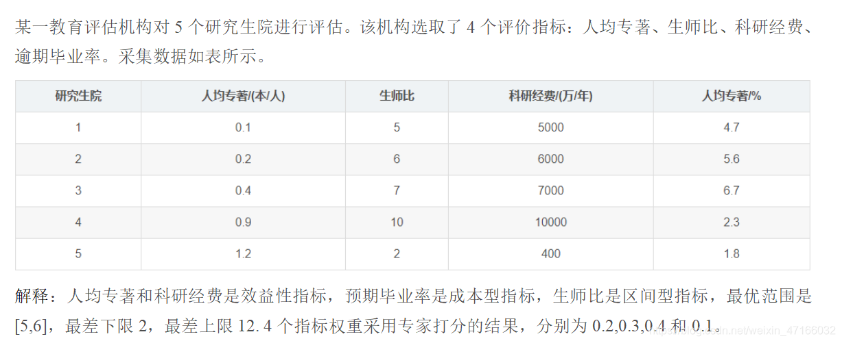
def data(file_path):
data = pd.read_excel(file_path).values
A = data[:, 1:]
A = np.array(A)
# m,n=A.shape[0],A.shape[1] #m表示行数,n表示列数
return A
# 权重
A = data('研究生院评估数据.xlsx')
A1 = standard(A)
C = Topsis(A1)
print(C)
熵值法
数据样本
import numpy as np
import pandas as pd
# 读取数据
data = pd.read_csv(r'C:\新建文件夹\data.csv', encoding='utf-8', index_col=0)
indicator = data.columns.tolist() # 指标个数
project = data.index.tolist() # 方案数、评价主体
value = data.values
data.head()
# 定义数据标准化函数。为了避免求熵值时对数无意义,对数据进行平移,对标准化后的数据统一加了常数0.001
def std_data(value,flag):
for i in range(len(indicator)):
if flag[i] == '+':
value[:, i] = (value[:, i]-np.min(value[:, i], axis=0))/(np.max(value[:, i], axis=0)-np.min(value[:, i], axis=0))+0.01
elif flag[i] == '-':
value[:, i] = (np.max(value[:, i], axis=0)-value[:, i])/(np.max(value[:, i], axis=0)-np.min(value[:, i], axis=0))+0.01
return value
# 数据标准化
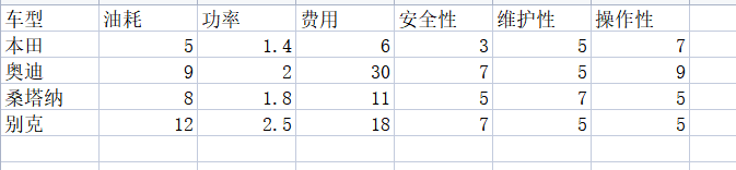
flag = ["-", "+", "-", "+", "+", "+"] # 表示指标为正向指标还是反向指标
std_value = std_data(value, flag)
std_value.round(3)
# 定义熵值法函数、熵值法计算变量的权重
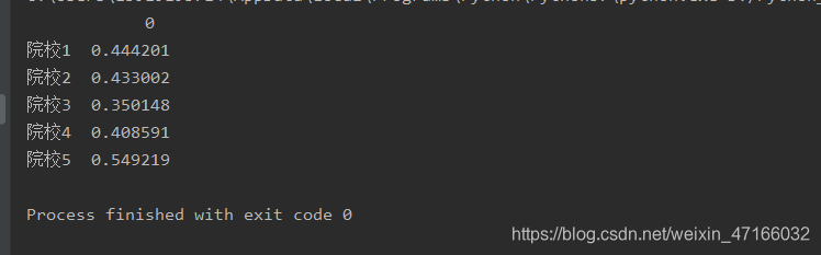
def cal_weight(indicator, project, value):
p = np.array([[0.0 for i in range(len(indicator))] for i in range(len(project))])
for i in range(len(indicator)):
p[:, i] = value[:, i] / np.sum(value[:, i], axis=0)
e = -1 / np.log(len(project)) * sum(p * np.log(p)) # 计算熵值
g = 1 - e # 计算一致性程度
w = g / sum(g) # 计算权重
return w
# 结果
w = cal_weight(indicator, project, std_value)
w = pd.DataFrame(w, index=data.columns, columns=['权重'])
print("#######权重:#######")
print(w)
score = np.dot(std_value, w).round(2)
score = pd.DataFrame(score, index=data.index, columns=['综合得分']).sort_values(by=['综合得分'], ascending=False)
print(score)
预测模型
回归拟合
最小二乘法(OLS)
最小二乘法是通过最小化样本真值与预测值之间的方差和来达到计算出 w 1 , w 2 , w 3 , . . , w n w_1,w_2,w_3,..,w_n w1,w2,w3,..,wn的目的。就是:
arg min ( ∑ ( y 1 − y ) 2 ) \argmin(\sum(y_1-y)^2) argmin(∑(y1−y)2)
其中 y 1 y_1 y1是样本预测值,y是样本中的真值。下面使用波士顿房价数据来实践拟合。
from sklearn import linear_model
import numpy as np
from sklearn.datasets import load_boston
from sklearn.model_selection import train_test_split

#  导入数据
boston = load_boston()
datas = boston.data
target = boston.target
name_data = boston.feature_names
#  选择特征进行训练
j_ = []
for i in range(13):
    if name_data[i] == 'RM':
        continue
    if name_data[i] =='LSTAT':
        continue
    j_.append(i)
x_data = np.delete(datas, j_, axis=1)
#  接下来把处理好的数据集分为训练集和测试集,选择线性回归模型训练与预测数据
X_train, X_test, y_train, y_test = train_test_split(x_data, target, random_state=0, test_size=0.20)
lr = linear_model.LinearRegression()
lr.fit(X_train, y_train)
lr_y_predict = lr.predict(X_test)
score = lr.score(X_test, y_test)
print(score)
print("w0:",lr.intercept_)
print("w1,w2:", lr.coef_)
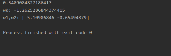
拟合到的线性模型是:y = -1.2625286844374415 + 5.10906846 x 1 x_1 x1 - 0.65494879 x 2 x_2 x2。
岭回归(Ridge Regression)
# encoding = 'utf-8'
import pandas as pd
from sklearn.model_selection import train_test_split
from sklearn.preprocessing import StandardScaler
from sklearn import linear_model
# 导入数据
data = pd.read_csv(r'C:\data\data.csv')
x_data = data.drop('y', 1)
x = x_data.drop('x11', 1)
y_data = data.loc[:, 'y']
name_data = list(data.columns.values)
# 数据预处理
train_data, test_data, train_target, test_target = train_test_split(x_data, y_data, test_size=0.3)
Stand_X = StandardScaler() # 特征进行标准化
Stand_Y = StandardScaler() # 标签也是数值,也需要进行标准化
train_data = Stand_X.fit_transform(train_data)
test_data = Stand_X.transform(test_data)
train_target = Stand_Y.fit_transform(train_target.values.reshape(-1, 1)) # reshape(-1,1)指将它转化为1列,行自动确定
test_target = Stand_Y.transform(test_target.values.reshape(-1, 1))
# 岭回归
rg = linear_model.Ridge(alpha=0.01)
rg.fit(train_data, train_target)
rg_score = rg.score(test_data, test_target)
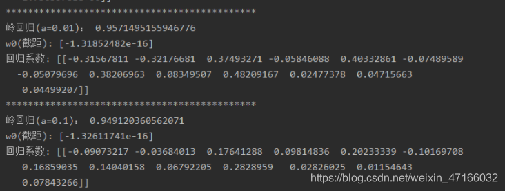
print("*********************************************")
print("岭回归(a=0.01):", rg_score)
print("w0(截距):", rg.intercept_)
print("回归系数:", rg.coef_)
# 岭回归
rg = linear_model.Ridge(alpha=0.1)
rg.fit(train_data, train_target)
rg_score = rg.score(test_data, test_target)
print("*********************************************")
print("岭回归(a=0.1):", rg_score)
print("w0(截距):", rg.intercept_)
print("回归系数:", rg.coef_)
LASSO回归
# encoding = 'utf-8'
import pandas as pd
from sklearn.model_selection import train_test_split
from sklearn.preprocessing import StandardScaler
from sklearn import linear_model
# 导入数据
data = pd.read_csv(r'C:\data\data.csv')
x_data = data.drop('y', 1)
x = x_data.drop('x11', 1)
y_data = data.loc[:, 'y']
name_data = list(data.columns.values)
# 数据预处理
train_data, test_data, train_target, test_target = train_test_split(x_data, y_data, test_size=0.3)
Stand_X = StandardScaler() # 特征进行标准化
Stand_Y = StandardScaler() # 标签也是数值,也需要进行标准化
train_data = Stand_X.fit_transform(train_data)
test_data = Stand_X.transform(test_data)
train_target = Stand_Y.fit_transform(train_target.values.reshape(-1, 1)) # reshape(-1,1)指将它转化为1列,行自动确定
test_target = Stand_Y.transform(test_target.values.reshape(-1, 1))
# Lasso回归
ls = linear_model.Lasso(alpha=0.01)
ls.fit(train_data, train_target)
ls_score = ls.score(test_data, test_target)
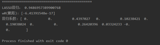
print("*********************************************")
print("LASSO回归:", ls_score)
print("w0(截距):", ls.intercept_)
print("回归系数:", ls.coef_)
如果不是很理解这几个回归模型,或者想了解这些模型的具体参数使用,可以看看这篇博文博文地址
灰色预测
# -*- coding: utf-8 -*-
"""
Spyder Editor

This is a temporary script file.
"""
import numpy as np
import math

history_data = [724.57, 746.62, 778.27, 800.8, 827.75, 871.1, 912.37, 954.28, 995.01, 1037.2]
n = len(history_data)
X0 = np.array(history_data)

#  累加生成
history_data_agg = [sum(history_data[0:i+1]) for i in range(n)]
X1 = np.array(history_data_agg)

#  计算数据矩阵B和数据向量Y
B = np.zeros([n-1, 2])
Y = np.zeros([n-1, 1])
for i in range(0, n-1):
    B[i][0] = -0.5*(X1[i] + X1[i+1])
    B[i][1] = 1
    Y[i][0] = X0[i+1]

#  计算GM(1,1)微分方程的参数a和u
#  A = np.zeros([2,1])
A = np.linalg.inv(B.T.dot(B)).dot(B.T).dot(Y)
a = A[0][0]
u = A[1][0]

#  建立灰色预测模型
XX0 = np.zeros(n)
XX0[0] = X0[0]
for i in range(1, n):
    XX0[i] = (X0[0] - u/a)*(1-math.exp(a))*math.exp(-a*(i))


#  模型精度的后验差检验
e = 0      # 求残差平均值
for i in range(0, n):
    e += (X0[i] - XX0[i])
e /= n

#  求历史数据平均值
aver = 0
for i in range(0, n):
    aver += X0[i]
aver /= n

#  求历史数据方差
s12 = 0
for i in range(0, n):
    s12 += (X0[i]-aver)**2
s12 /= n

#  求残差方差
s22 = 0
for i in range(0, n):
    s22 += ((X0[i] - XX0[i]) - e)**2
s22 /= n

#  求后验差比值
C = s22 / s12

#  求小误差概率
cout = 0
for i in range(0, n):
    if abs((X0[i] - XX0[i]) - e) < 0.6754*math.sqrt(s12):
        cout = cout+1
    else:
        cout = cout
P = cout / n

if (C < 0.35 and P > 0.95):
    # 预测精度为一级
    m = 10   # 请输入需要预测的年数
    f = np.zeros(m)
    for i in range(0, m):
        f[i] = (X0[0] - u/a)*(1-math.exp(a))*math.exp(-a*(i+n))
else:
    print('灰色预测法不适用')
马尔可夫预测
'''
  https://github.com/hmmlearn/hmmlearn
  hmm包
  来源于https://blog.csdn.net/xinfeng2005/article/details/53939192
  GaussianHMM是针对观测为连续,所以观测矩阵B由各个隐藏状态对应观测状态的高斯分布概率密度函数参数来给出
  对应GMMHMM同样,而multinomialHMM是针对离散观测,B可以直接给出
'''
from hmmlearn.hmm import GaussianHMM
from hmmlearn.hmm import MultinomialHMM

#  观测状态是二维,而隐藏状态有4个。
#  因此我们的“means”参数是4×24×2的矩阵,而“covars”参数是4×2×24×2×2的张量
import numpy as np
startprob = np.array([0.6, 0.3, 0.1, 0.0])
#  这里1,3之间无转移可能,对应矩阵为0?
transmat = np.array([[0.7, 0.2, 0.0, 0.1],
                     [0.3, 0.5, 0.2, 0.0],
                     [0.0, 0.3, 0.5, 0.2],
                     [0.2, 0.0, 0.2, 0.6]])
# 隐藏状态(component)高斯分布均值?The means of each component
means = np.array([[0.0,  0.0],
                  [0.0, 11.0],
                  [9.0, 10.0],
                  [11.0, -1.0]])
# 隐藏状态协方差The covariance of each component
covars = .5*np.tile(np.identity(2),(4,1,1))
# np.tile(x,(n,m)),将x延第一个轴复制n个出来,再延第二个轴复制m个出来。上面,为1*2*2,复制完了就是4*2*2
#np.identity(n)获取n维单位方阵,np.eye(n.m.k)获取n行m列对角元素偏移k的单位阵
'''
参数covariance_type,为"full":所有的μ,Σ都需要指定。取值为“spherical”则Σ的非对角线元素为0,对角线元素相同。
取值为“diag”则Σ的非对角线元素为0,对角线元素可以不同,"tied"指所有的隐藏状态对应的观测状态分布使用相同的协方差矩阵Σ
'''
hmm = GaussianHMM(n_components=4,
                covariance_type='full',
                startprob_prior=1.0,  # PI
                transmat_prior=1.0,  # 状态转移A
                means_prior=means,  # “means”用来表示各个隐藏状态对应的高斯分布期望向量μ形成的矩阵
                means_weight=1,
                covars_prior=covars,  # “covars”用来表示各个隐藏状态对应的高斯分布协方差矩阵Σ形成的三维张量
                covars_weight=1,
                algorithm=1,
                )
hmm = GaussianHMM(n_components=4, covariance_type='full')
# 我们不是从数据中拟合,而是直接设置估计参数、分量的均值和协方差
hmm.startprob_ = startprob
hmm.transmat_ = transmat
hmm.means_ = means
hmm.covars_ = covars
# 以上,构建(训练)好了HMM模型(这里没有训练直接给定参数,需要训练则fit)
# 观测状态二维,使用三维观测序列,输入3*2*2张量
seen = np.array([[1.1, 2.0], [-1, 2.0], [3, 7]])
logprob, state = hmm.decode(seen, algorithm="viterbi")
print(state)
# HMM问题1对数概率计算
print(hmm.score(seen))
时间序列分析
import pandas
import matplotlib.pyplot as plt
from statsmodels.graphics.tsaplots import plot_acf
from statsmodels.tsa.stattools import adfuller as ADF
from statsmodels.graphics.tsaplots import plot_pacf
from statsmodels.stats.diagnostic import acorr_ljungbox
from statsmodels.tsa.arima_model import ARIMA

# 读取数据,指定日期为索引列
data = pandas.read_csv(
    'D:\\DATA\\pycase\\number2\\9.3\\Data.csv',
    index_col='日期'
)

# 绘图过程中
# 用来正常显示中文标签
plt.rcParams['font.sans-serif']=['SimHei']

# 用来正常显示负号

plt.rcParams['axes.unicode_minus'] = False

# 查看趋势图
data.plot()  # 有增长趋势,不平稳
# 附加:查看自相关系数合片自相关系数(查分之后),可以用于平稳性的检测,也可用于定阶系数预估
# 自相关图()
plot_acf(data).show()  # 自相关图既不是拖尾也不是截尾。以上的图的自相关是一个三角对称的形式,这种趋势是单调趋势的典型图形,说明这个序列不是平稳序列


# 1 平稳性检测
def tagADF(t):
    result=pandas.DataFrame(index=[
        "Test Statistic Value", "p-value", "Lags Used",
        "Number of Observations Used",
        "Critical Value(1%)", "Critical Value(5%)", "Critical Value(10%)"
    ], columns=['销量']
    )
    result['销量']['Test Statistic Value'] = t[0]
    result['销量']['p-value'] = t[1]
    result['销量']['Lags Used'] = t[2]
    result['销量']['Number of Observations Used'] = t[3]
    result['销量']['Critical Value(1%)'] = t[4]['1%']
    result['销量']['Critical Value(5%)'] = t[4]['5%']
    result['销量']['Critical Value(10%)'] = t[4]['10%']
    return result


print('原始序列的ADF检验结果为:', tagADF(ADF(data[u'销量'])))  # 添加标签后展现

# 平稳判断:得到统计量大于三个置信度(1%,5%,10%)临界统计值,p值显著大于0.05,该序列为非平稳序列。
# 备注:得到的统计量显著小于3个置信度(1%,5%,10%)的临界统计值时,为平稳 此时p值接近于0 此处不为0,尝试增加数据量,原数据太少

# 2 进行数据差分,一般一阶差分就可以
D_data = data.diff(1).dropna()
D_data.columns = [u'销量差分']

# 差分图趋势查看
D_data.plot()
plt.show()

# 附加:查看自相关系数合片自相关系数(查分之后),可以用于平稳性的检测,也可用于定阶系数预估

# 自相关图
plot_acf(D_data).show()
plt.show()
# 偏自相关图
plot_pacf(D_data).show()

# 3 平稳性检测
print(u'差分序列的ADF检验结果为:', tagADF(ADF(D_data[u'销量差分'])))
# 解释:Test Statistic Value值小于两个水平值,p值显著小于0.05,一阶差分后序列为平稳序列。

# 4 白噪声检验
# 返回统计量和p值
print(u'差分序列的白噪声检验结果为:', acorr_ljungbox(D_data, lags=1))  # 分别为stat值(统计量)和P值
# P值小于0.05,所以一阶差分后的序列为平稳非白噪声序列。

# 5 p,q定阶
# 一般阶数不超过length/10
pmax = int(len(D_data) / 10)
# 一般阶数不超过length/10
qmax = int(len(D_data) / 10)

# bic矩阵
bic_matrix = []
for p in range(pmax + 1):
    tmp = []
    for q in range(qmax + 1):
        # 存在部分报错,所以用try来跳过报错。
        try:
            tmp.append(ARIMA(data, (p, 1, q)).fit().bic)
        except:
            tmp.append(None)
    bic_matrix.append(tmp)

# 从中可以找出最小值
bic_matrix = pandas.DataFrame(bic_matrix)
# 先用stack展平,然后用idxmin找出最小值位置。
p, q = bic_matrix.stack().idxmin()

print(u'BIC最小的p值和q值为:%s、%s' % (p, q))
# 取BIC信息量达到最小的模型阶数,结果p为0,q为1,定阶完成。

# 6 建立模型和预测
model = ARIMA(data, (p, 1, q)).fit()
# 给出一份模型报告
model.summary2()
# 作为期5天的预测,返回预测结果、标准误差、置信区间。
model.forecast(5)
支持向量机(svm)
svm常用的有四种核函数:1. 线性核函数,2.高斯核函数,3.多项式核函数,4.sigmoid核函数。具体没有那种场景绝对使用某个核函数,它们在大多数情况下表现差别不大,每种核函数在特定的数据集上的表现依赖于调整合适的超参数。
from sklearn.datasets import load_boston
from sklearn.preprocessing import StandardScaler
from sklearn.model_selection import train_test_split
from sklearn.svm import LinearSVR
from sklearn.svm import SVR

# 导入数据集
boston = load_boston()
data = boston.data
target = boston.target
# 数据预处理
train_data, test_data, train_target, test_target = train_test_split(data, target, test_size=0.3)
Stand_X = StandardScaler()  # 特征进行标准化
Stand_Y = StandardScaler()  # 标签也是数值,也需要进行标准化
train_data = Stand_X.fit_transform(train_data)
test_data = Stand_X.transform(test_data)
train_target = Stand_Y.fit_transform(train_target.reshape(-1, 1))  # reshape(-1,1)指将它转化为1列,行自动确定
test_target = Stand_Y.transform(test_target.reshape(-1, 1))
#  线性核函数
clf = LinearSVR(C=2)
clf.fit(train_data, train_target)
print("线性核函数:")
print("测试集评分:", clf.score(train_data, train_target))
print("测试数据到超平面的距离(返回前五个)", clf._decision_function(test_data)[:5])
print("测试集预测结果(前5个):", clf.predict(test_data)[:5])
#  高斯核函数
clf = SVR(kernel='rbf', C=10, gamma=0.1, coef0=0.1)
clf.fit(train_data, train_target)
print("高斯核函数:")
print("测试集评分:", clf.score(test_data, test_target))
print("测试数据到超平面的距离(返回前五个)", clf._decision_function(test_data)[:5])
print("测试集预测结果(前5个):", clf.predict(test_data)[:5])
#  sigmoid核函数
clf = SVR(kernel='sigmoid', C=2)
clf.fit(train_data, train_target)
print("sigmoid核函数:")
print("测试集评分:", clf.score(test_data, test_target))
print("测试数据到超平面的距离(返回前五个)", clf._decision_function(test_data)[:5])
print("测试集预测结果(前5个):", clf.predict(test_data)[:5])
#  多项式核函数
clf = SVR(kernel='poly', C=2)
clf.fit(train_data, train_target)
print("多项式核函数:")
print("测试集评分:", clf.score(test_data, test_target))
print("测试数据到超平面的距离(返回前五个)", clf._decision_function(test_data)[:5])
print("测试集预测结果(前5个):", clf.predict(test_data)[:5])
决策树
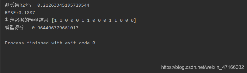
数据集用的是数学建模比赛——2021年第二届“华数杯”全国大学生数学建模c题的数据。具体的参数调用可以查看这篇博文地址。树的可视化需要另外安装插件,具体安装可以看这篇博文地址。
# encoding = 'utf-8' python=3.76
import numpy as np
import pandas as pd
from sklearn.model_selection import train_test_split
from sklearn import metrics
from sklearn.metrics import mean_squared_error
from math import sqrt
from sklearn import tree
import graphviz
import pydotplus
import os

# 导入数据
data = pd.read_excel('C:\\Users\\新建文件夹\\目标客户体验数据(清洗).xlsx')
test_data = pd.read_excel('C:\\Users\\新建文件夹\\待判定的数据.xlsx')
# 清洗数据,筛选特征a1到a8和特征B13,B15,B16, B17
x_test = test_data.drop('是否会购买?', 1)
x_test1 = x_test.drop(['客户编号', '品牌编号 ', 'B1', 'B2', 'B3', 'B4', 'B5', 'B6', 'B7', 'B8', 'B9', 'B10', 'B11', 'B12', 'B14'], 1)
x_data = data.drop('购买意愿', 1)
x_data1 = x_data.drop(['目标客户编号', '品牌类型', 'B1', 'B2', 'B3', 'B4', 'B5', 'B6', 'B7', 'B8', 'B9', 'B10', 'B11', 'B12', 'B14'], 1)
y_data = data.loc[:, '购买意愿']
name_data = list(data.columns.values)
# 把清洗好的数据拆分成训练集和测试集
train_data, test_data, train_target, test_target = train_test_split(x_data1, y_data, test_size=0.3)
# 决策树
clf = tree.DecisionTreeClassifier(criterion="gini",
                 splitter="best",
                 max_depth=4,
                 min_samples_split=2,
                 min_samples_leaf=7,
                 min_weight_fraction_leaf=0.,
                 max_features=None,
                 random_state=None,
                 max_leaf_nodes=None,
                 min_impurity_decrease=0.,
                 min_impurity_split=None,
                 class_weight=None,
                 presort=False)

clf.fit(train_data, train_target.astype('int'))  # 使用训练集训练模型
y_pred = clf.predict(test_data)
predict_results = clf.predict(x_test1)  # 使用模型对待判定数据进行预测
scores = clf.score(test_data, test_target.astype('int'))
MSE = np.sum((y_pred-test_target)**2)/len(test_target)
print("测试集R2分:", metrics.r2_score(test_target, y_pred.reshape(-1, 1)))
print('RMSE:{:.4f}'.format(sqrt(MSE)))  # RMSE(标准误差)
print("判定数据的预测结果", predict_results)
print("模型得分:", scores)
# 可视化树并保存
os.environ["PATH"] += os.pathsep + r'C:\Program Files\Graphviz\bin'
with open("tree.dot", 'w') as f:
    f = tree.export_graphviz(clf, out_file=f)
dot_data = tree.export_graphviz(clf, out_file=None, feature_names=[u'a1', u'a2', u'a3', u'a4', u'a5', u'a6', u'a7', u'a8', u'B13', u'B15', u'B16', u'B17'],
                                 class_names=[u'0', u'1'], filled=True, rotate=True)
graph = pydotplus.graph_from_dot_data(dot_data)
# 保存图像为pdf文件
graph.write_pdf("tree.pdf")

随机森林
"""
随机森林需要调整的参数有:
(1) 决策树的个数
(2) 特征属性的个数
(3) 递归次数(即决策树的深度)
"""
from numpy import inf
from numpy import zeros
import numpy as np
from sklearn.model_selection import train_test_split
# 生成数据集。数据集包括标签,全包含在返回值的dataset上
def get_Datasets():
from sklearn.datasets import make_classification
dataSet, classLabels = make_classification(n_samples=200, n_features=100, n_classes=2)
return np.concatenate((dataSet, classLabels.reshape((-1, 1))), axis=1)
'''
切分数据集,实现交叉验证。可以利用它来选择决策树个数。但本例没有实现其代码。
原理如下:
第一步,将训练集划分为大小相同的K份;
第二步,我们选择其中的K-1分训练模型,将用余下的那一份计算模型的预测值,
这一份通常被称为交叉验证集;第三步,我们对所有考虑使用的参数建立模型
并做出预测,然后使用不同的K值重复这一过程。
然后是关键,我们利用在不同的K下平均准确率最高所对应的决策树个数
作为算法决策树个数
'''
def splitDataSet(dataSet,n_folds): # 将训练集划分为大小相同的n_folds份;
fold_size = len(dataSet)/n_folds
data_split = []
begin = 0
end = fold_size
for i in range(n_folds):
data_split.append(dataSet[begin:end, :])
begin = end
end += fold_size
return data_split
# 构建n个子集
def get_subsamples(dataSet, n):
subDataSet = []
for i in range(n):
index = [] # 每次都重新选择k个 索引
for k in range(len(dataSet)): # 长度是k
index.append(np.random.randint(len(dataSet))) # (0,len(dataSet)) 内的一个整数
subDataSet.append(dataSet[index, :])
return subDataSet
# 根据某个特征及值对数据进行分类
def binSplitDataSet(dataSet, feature, value):
mat0 = dataSet[np.nonzero(dataSet[:, feature] > value)[0], :]
mat1 = dataSet[np.nonzero(dataSet[:, feature] < value)[0], :]
return mat0,mat1
feature = 2
value = 1
dataSet = get_Datasets()
mat0, mat1 = binSplitDataSet(dataSet, 2, 1)
# 计算方差,回归时使用
def regErr(dataSet):
return np.var(dataSet[:, -1])*np.shape(dataSet)[0]
# 计算平均值,回归时使用
def regLeaf(dataSet):
return np.mean(dataSet[:, -1])
def MostNumber(dataSet): # 返回多类
len0 = len(np.nonzero(dataSet[:, -1] == 0)[0])
len1 = len(np.nonzero(dataSet[:, -1] == 1)[0])
if len0>len1:
return 0
else:
return 1
# 计算基尼指数 一个随机选中的样本在子集中被分错的可能性 是被选中的概率乘以被分错的概率
def gini(dataSet):
corr = 0.0
for i in set(dataSet[:,-1]): # i是这个特征下的 某个特征值
corr += (len(np.nonzero(dataSet[:, -1] == i)[0])/len(dataSet))**2
return 1-corr
def select_best_feature(dataSet, m, alpha="huigui"):
f = dataSet.shape[1] # 拿过这个数据集,看这个数据集有多少个特征,即f个
index = []
bestS = inf
bestfeature = 0
bestValue = 0
if alpha == "huigui":
S = regErr(dataSet)
else:
S = gini(dataSet)
for i in range(m):
index.append(np.random.randint(f)) # 在f个特征里随机,注意是随机!选择m个特征,然后在这m个特征里选择一个合适的分类特征。
for feature in index:
for splitVal in set(dataSet[:, feature]): # set() 函数创建一个无序不重复元素集,用于遍历这个特征下所有的值
mat0, mat1 = binSplitDataSet(dataSet, feature, splitVal)
if alpha == "huigui": newS = regErr(mat0)+regErr(mat1) # 计算每个分支的回归方差
else:
newS = gini(mat0)+gini(mat1) # 计算被分错率
if bestS > newS:
bestfeature = feature
bestValue = splitVal
bestS = newS
if (S-bestS) < 0.001 and alpha == "huigui": # 对于回归来说,方差足够了,那就取这个分支的均值
return None, regLeaf(dataSet)
elif (S-bestS) < 0.001:
return None, MostNumber(dataSet) # 对于分类来说,被分错率足够下了,那这个分支的分类就是大多数所在的类。
return bestfeature, bestValue
def createTree(dataSet, alpha="huigui", m=20, max_level=10): # 实现决策树,使用20个特征,深度为10,
bestfeature, bestValue = select_best_feature(dataSet, m, alpha=alpha)
if bestfeature == None:
return bestValue
retTree = {
}
max_level -= 1
if max_level < 0: # 控制深度
return regLeaf(dataSet)
retTree['bestFeature'] = bestfeature
retTree['bestVal'] = bestValue
lSet, rSet = binSplitDataSet(dataSet, bestfeature, bestValue) # lSet是根据特征bestfeature分到左边的向量,rSet是根据特征bestfeature分到右边的向量
retTree['right'] = createTree(rSet, alpha, m, max_level)
retTree['left'] = createTree(lSet, alpha, m, max_level) # 每棵树都是二叉树,往下分类都是一分为二。
return retTree
def RondomForest(dataSet, n, alpha="huigui"): # 树的个数
Trees = [] # 设置一个空树集合
for i in range(n):
X_train, X_test, y_train, y_test = train_test_split(dataSet[:,:-1], dataSet[:, -1], test_size=0.33, random_state=42)
X_train = np.concatenate((X_train, y_train.reshape((-1, 1))), axis=1)
Trees.append(createTree(X_train, alpha=alpha))
return Trees # 生成好多树
# 预测单个数据样本,重头!!如何利用已经训练好的随机森林对单个样本进行 回归或分类!
def treeForecast(trees, data, alpha="huigui"):
if alpha == "huigui":
if not isinstance(trees, dict): # isinstance() 函数来判断一个对象是否是一个已知的类型
return float(trees)
if data[trees['bestFeature']] > trees['bestVal']: # 如果数据的这个特征大于阈值,那就调用左支
if type(trees['left']) == 'float': # 如果左支已经是节点了,就返回数值。如果左支还是字典结构,那就继续调用, 用此支的特征和特征值进行选支。
return trees['left']
else:
return treeForecast(trees['left'], data, alpha)
else:
if type(trees['right']) == 'float':
return trees['right']
else:
return treeForecast(trees['right'], data, alpha)
else:
if not isinstance(trees, dict): # 分类和回归是同一道理
return int(trees)
if data[trees['bestFeature']] > trees['bestVal']:
if type(trees['left']) == 'int':
return trees['left']
else:
return treeForecast(trees['left'], data, alpha)
else:
if type(trees['right']) == 'int':
return trees['right']
else:
return treeForecast(trees['right'], data, alpha)
# 随机森林 对 数据集打上标签 0、1 或者是 回归值
def createForeCast(trees, test_dataSet, alpha="huigui"):
cm = len(test_dataSet)
yhat = np.mat(zeros((cm, 1)))
for i in range(cm):
yhat[i, 0] = treeForecast(trees, test_dataSet[i, :], alpha)
return yhat
# 随机森林预测
def predictTree(Trees, test_dataSet, alpha="huigui"): # trees 是已经训练好的随机森林 调用它!
cm = len(test_dataSet)
yhat = np.mat(zeros((cm, 1)))
for trees in Trees:
yhat += createForeCast(trees, test_dataSet, alpha) # 把每次的预测结果相加
if alpha == "huigui": yhat /= len(Trees) # 如果是回归的话,每棵树的结果应该是回归值,相加后取平均
else:
for i in range(len(yhat)): # 如果是分类的话,每棵树的结果是一个投票向量,相加后,
# 看每类的投票是否超过半数,超过半数就确定为1
if yhat[i, 0] > len(Trees)/2:
yhat[i, 0] = 1
else:
yhat[i, 0] = 0
return yhat
if __name__ == '__main__':
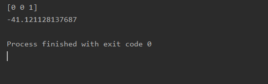
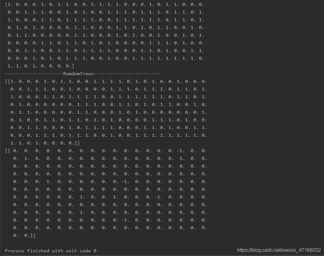
dataSet = get_Datasets()
print(dataSet[:, -1].T) # 打印标签,与后面预测值对比 .T其实就是对一个矩阵的转置
RomdomTrees = RondomForest(dataSet, 4, alpha="fenlei") # 这里我训练好了 很多树的集合,就组成了随机森林。一会一棵一棵的调用。
print("---------------------RomdomTrees------------------------")
test_dataSet = dataSet # 得到数据集和标签
yhat = predictTree(RomdomTrees, test_dataSet, alpha="fenlei") # 调用训练好的那些树。综合结果,得到预测值。
print(yhat.T)
# get_Datasets()
print(dataSet[:, -1].T-yhat.T)
图论模型
最短路径
# 找到一条从start到end的路径
def findPath(graph, start, end, path=[]):
path = path + [start]
if start == end:
return path
for node in graph[start]:
if node not in path:
newpath = findPath(graph, node, end, path)
if newpath:
return newpath
return None
# 找到所有从start到end的路径
def findAllPath(graph, start, end, path=[]):
path = path + [start]
if start == end:
return [path]
paths = [] # 存储所有路径
for node in graph[start]:
if node not in path:
newpaths = findAllPath(graph, node, end, path)
for newpath in newpaths:
paths.append(newpath)
return paths
# 查找最短路径
def findShortestPath(graph, start, end, path=[]):
path=path + [start]
if start == end:
return path
shortestPath = []
for node in graph[start]:
if node not in path:
newpath = findShortestPath(graph, node, end, path)
if newpath:
if not shortestPath or len(newpath) < len(shortestPath):
shortestPath = newpath
return shortestPath
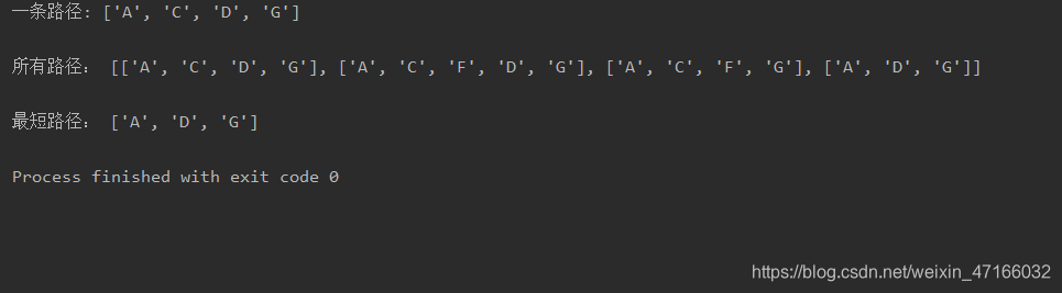
graph = {
'A': ['B', 'C', 'D'],
'B': ['E'],
'C': ['D', 'F'],
'D': ['B', 'E', 'G'],
'E': [],
'F': ['D', 'G'],
'G': ['E']}
onepath = findPath(graph, 'A', 'G')
print('一条路径:', onepath)
allpath = findAllPath(graph, 'A', 'G')
print('\n所有路径:', allpath)
shortpath = findShortestPath(graph, 'A', 'G')
print('\n最短路径:', shortpath)
最小生成树
这里引用的是这篇博文添加链接描述
# mathmodel18_v1.py
# Demo18 of mathematical modeling algorithm
# Demo of minimum spanning tree(MST) with NetworkX
# Copyright 2021 YouCans, XUPT
# Crated:2021-07-10
import numpy as np
import matplotlib.pyplot as plt
import networkx as nx
# 1. 天然气管道铺设
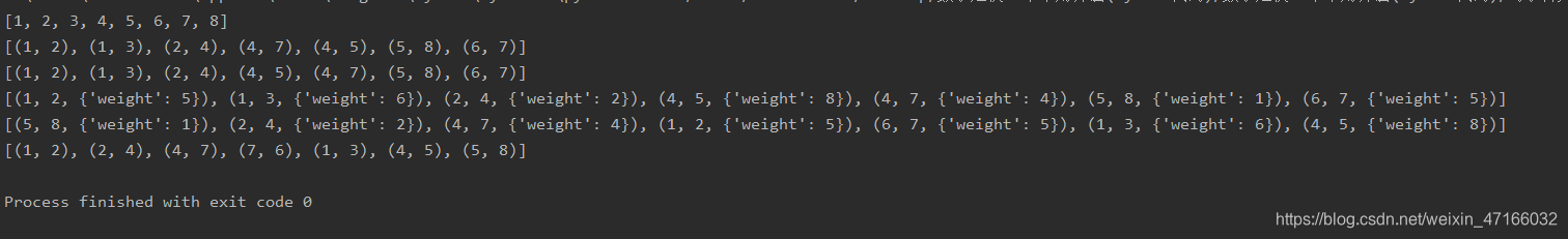
G1 = nx.Graph() # 创建:空的 无向图
G1.add_weighted_edges_from([(1, 2, 5), (1, 3, 6), (2, 4, 2), (2, 5, 12), (3, 4, 6),
(3, 6, 7), (4, 5, 8), (4, 7, 4), (5, 8, 1), (6, 7, 5), (7, 8, 10)]) # 向图中添加多条赋权边: (node1,node2,weight)
T = nx.minimum_spanning_tree(G1) # 返回包括最小生成树的图
print(T.nodes) # 最小生成树的 顶点
print(T.edges) # 最小生成树的 边
print(sorted(T.edges)) # 排序后的 最小生成树的 边
print(sorted(T.edges(data=True))) # data=True 表示返回值包括边的权重
mst1 = nx.tree.minimum_spanning_edges(G1, algorithm="kruskal") # 返回最小生成树的边
print(list(mst1)) # 最小生成树的 边
mst2 = nx.tree.minimum_spanning_edges(G1, algorithm="prim", data=False) # data=False 表示返回值不带权
print(list(mst2))
# 绘图
pos = {
1: (1, 5), 2: (3, 1), 3: (3, 9), 4: (5, 5), 5: (7, 1), 6: (6, 9), 7: (8, 7), 8: (9, 4)} # 指定顶点位置
nx.draw(G1, pos, with_labels=True, node_color='c', alpha=0.8) # 绘制无向图
labels = nx.get_edge_attributes(G1, 'weight')
nx.draw_networkx_edge_labels(G1, pos, edge_labels=labels, font_color='m') # 显示边的权值
nx.draw_networkx_edges(G1, pos, edgelist=T.edges, edge_color='b', width=4) # 设置指定边的颜色
plt.show()

旅行商问题
模拟退火算法
# 模拟退火算法求解旅行商问题 Python程序
# 程序来源:https://blog.csdn.net/youcans/article/details/116396137
# 模拟退火求解旅行商问题(TSP)基本算法
# -*- coding: utf-8 -*-
import math
import random
import pandas as pd
import numpy as np
import matplotlib.pyplot as plt
np.set_printoptions(precision=4)
pd.set_option('display.max_rows', 20)
pd.set_option('expand_frame_repr', False)
pd.options.display.float_format = '{:,.2f}'.format
# 子程序:初始化模拟退火算法的控制参数
def initParameter():
tInitial = 100.0 # 设定初始退火温度(initial temperature)
tFinal = 1 # 设定终止退火温度(stop temperature)
nMarkov = 1000 # Markov链长度,也即内循环运行次数
alfa = 0.98 # 设定降温参数,T(k)=alfa*T(k-1)
return tInitial, tFinal, alfa, nMarkov
# 子程序:读取TSPLib数据
def read_TSPLib(fileName):
res = []
with open(fileName, 'r') as fid:
for item in fid:
if len(item.strip()) != 0:
res.append(item.split())
loadData = np.array(res).astype('int') # 数据格式:i Xi Yi
coordinates = loadData[:, 1::]
return coordinates
# 子程序:计算各城市间的距离,得到距离矩阵
def getDistMat(nCities, coordinates):
distMat = np.zeros((nCities, nCities)) # 初始化距离矩阵
for i in range(nCities):
for j in range(i, nCities):
# np.linalg.norm 求向量的范数(默认求 二范数),得到 i、j 间的距离
distMat[i][j] = distMat[j][i] = round(np.linalg.norm(coordinates[i]-coordinates[j]))
return distMat # 城市间距离取整(四舍五入)
# 子程序:计算 TSP 路径长度
def calTourMileage(tourGiven, nCities, distMat):
mileageTour = distMat[tourGiven[nCities-1], tourGiven[0]] # dist((n-1),0)
for i in range(nCities-1): # dist(0,1),...dist((n-2)(n-1))
mileageTour += distMat[tourGiven[i], tourGiven[i+1]]
return round(mileageTour) # 路径总长度取整(四舍五入)
# 子程序:绘制 TSP 路径图
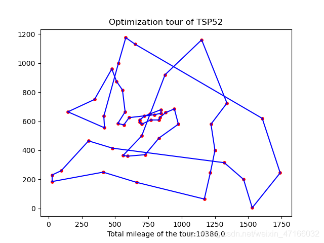
def plot_tour(tour, value, coordinates):
# custom function plot_tour(tour, nCities, coordinates)
num = len(tour)
x0, y0 = coordinates[tour[num - 1]]
x1, y1 = coordinates[tour[0]]
plt.scatter(int(x0), int(y0), s=15, c='r') # 绘制城市坐标点 C(n-1)
plt.plot([x1, x0], [y1, y0], c='b') # 绘制旅行路径 C(n-1)~C(0)
for i in range(num - 1):
x0, y0 = coordinates[tour[i]]
x1, y1 = coordinates[tour[i + 1]]
plt.scatter(int(x0), int(y0), s=15, c='r') # 绘制城市坐标点 C(i)
plt.plot([x1, x0], [y1, y0], c='b') # 绘制旅行路径 C(i)~C(i+1)
plt.xlabel("Total mileage of the tour:{:.1f}".format(value))
plt.title("Optimization tour of TSP{:d}".format(num)) # 设置图形标题
plt.show()
# 子程序:交换操作算子
def mutateSwap(tourGiven, nCities):
# 在 [0,n) 产生 2个不相等的随机整数 i,j
i = np.random.randint(nCities) # 产生第一个 [0,n) 区间内的随机整数
while True:
j = np.random.randint(nCities) # 产生一个 [0,n) 区间内的随机整数
if i != j: break # 保证 i, j 不相等
tourSwap = tourGiven.copy() # 将给定路径复制给新路径 tourSwap
tourSwap[i], tourSwap[j] = tourGiven[j], tourGiven[i] # 交换 城市 i 和 j 的位置————简洁的实现方法
return tourSwap
def main():
# 读取旅行城市位置的坐标
coordinates = np.array([[565.0, 575.0], [25.0, 185.0], [345.0, 750.0], [945.0, 685.0], [845.0, 655.0],
[880.0, 660.0], [25.0, 230.0], [525.0, 1000.0], [580.0, 1175.0], [650.0, 1130.0],
[1605.0, 620.0], [1220.0, 580.0], [1465.0, 200.0], [1530.0, 5.0], [845.0, 680.0],
[725.0, 370.0], [145.0, 665.0], [415.0, 635.0], [510.0, 875.0], [560.0, 365.0],
[300.0, 465.0], [520.0, 585.0], [480.0, 415.0], [835.0, 625.0], [975.0, 580.0],
[1215.0, 245.0], [1320.0, 315.0], [1250.0, 400.0], [660.0, 180.0], [410.0, 250.0],
[420.0, 555.0], [575.0, 665.0], [1150.0, 1160.0], [700.0, 580.0], [685.0, 595.0],
[685.0, 610.0], [770.0, 610.0], [795.0, 645.0], [720.0, 635.0], [760.0, 650.0],
[475.0, 960.0], [95.0, 260.0], [875.0, 920.0], [700.0, 500.0], [555.0, 815.0],
[830.0, 485.0], [1170.0, 65.0], [830.0, 610.0], [605.0, 625.0], [595.0, 360.0],
[1340.0, 725.0], [1740.0, 245.0]])
# fileName = "../data/eil76.dat" # 数据文件的地址和文件名
# coordinates = read_TSPLib(fileName) # 调用子程序,读取城市坐标数据文件
# 模拟退火算法参数设置
tInitial, tFinal, alfa, nMarkov = initParameter() # 调用子程序,获得设置参数
nCities = coordinates.shape[0] # 根据输入的城市坐标 获得城市数量 nCities
distMat = getDistMat(nCities, coordinates) # 调用子程序,计算城市间距离矩阵
nMarkov = nCities # Markov链 的初值设置
tNow = tInitial # 初始化 当前温度(current temperature)
# 初始化准备
tourNow = np.arange(nCities) # 产生初始路径,返回一个初值为0、步长为1、长度为n 的排列
valueNow = calTourMileage(tourNow, nCities, distMat) # 计算当前路径的总长度 valueNow
tourBest = tourNow.copy() # 初始化最优路径,复制 tourNow
valueBest = valueNow # 初始化最优路径的总长度,复制 valueNow
recordBest = [] # 初始化 最优路径记录表
recordNow = [] # 初始化 最优路径记录表
# 开始模拟退火优化过程
iter = 0 # 外循环迭代次数计数器
while tNow >= tFinal: # 外循环,直到当前温度达到终止温度时结束
# 在当前温度下,进行充分次数(nMarkov)的状态转移以达到热平衡
for k in range(nMarkov): # 内循环,循环次数为Markov链长度
# 产生新解:
tourNew = mutateSwap(tourNow, nCities) # 通过 交换操作 产生新路径
valueNew = calTourMileage(tourNew, nCities, distMat) # 计算当前路径的总长度
deltaE = valueNew - valueNow
# 接受判别:按照 Metropolis 准则决定是否接受新解
if deltaE < 0: # 更优解:如果新解的目标函数好于当前解,则接受新解
accept = True
if valueNew < valueBest: # 如果新解的目标函数好于最优解,则将新解保存为最优解
tourBest[:] = tourNew[:]
valueBest = valueNew
else: # 容忍解:如果新解的目标函数比当前解差,则以一定概率接受新解
pAccept = math.exp(-deltaE/tNow) # 计算容忍解的状态迁移概率
if pAccept > random.random():
accept = True
else:
accept = False
# 保存新解
if accept == True: # 如果接受新解,则将新解保存为当前解
tourNow[:] = tourNew[:]
valueNow = valueNew
# 平移当前路径,以解决变换操作避开 0,(n-1)所带来的问题,并未实质性改变当前路径。
tourNow = np.roll(tourNow, 2) # 循环移位函数,沿指定轴滚动数组元素
# 完成当前温度的搜索,保存数据和输出
recordBest.append(valueBest) # 将本次温度下的最优路径长度追加到 最优路径记录表
recordNow.append(valueNow) # 将当前路径长度追加到 当前路径记录表
print('i:{}, t(i):{:.2f}, valueNow:{:.1f}, valueBest:{:.1f}'.format(iter, tNow, valueNow, valueBest))
# 缓慢降温至新的温度,
iter = iter + 1
tNow = tNow * alfa # 指数降温曲线:T(k)=alfa*T(k-1)
# 结束模拟退火过程
# 图形化显示优化结果
figure1 = plt.figure() # 创建图形窗口 1
plot_tour(tourBest, valueBest, coordinates)
figure2 = plt.figure() # 创建图形窗口 2
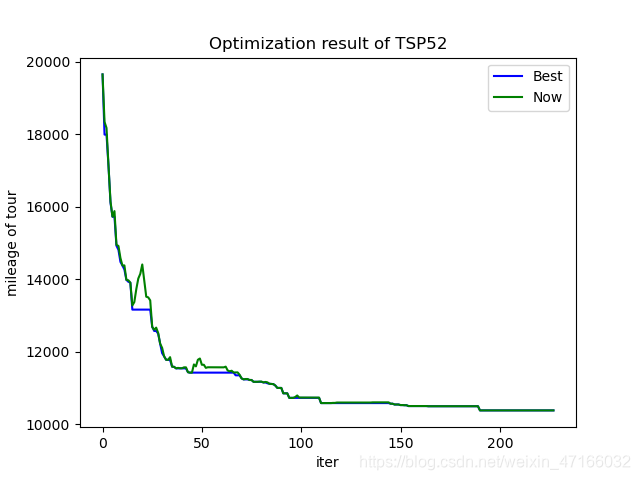
plt.title("Optimization result of TSP{:d}".format(nCities)) # 设置图形标题
plt.plot(np.array(recordBest),'b-', label='Best') # 绘制 recordBest曲线
plt.plot(np.array(recordNow),'g-', label='Now') # 绘制 recordNow曲线
plt.xlabel("iter") # 设置 x轴标注
plt.ylabel("mileage of tour") # 设置 y轴标注
plt.legend() # 显示图例
plt.show()
print("Tour verification successful!")
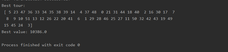
print("Best tour: \n", tourBest)
print("Best value: {:.1f}".format(valueBest))
exit()
if __name__ == '__main__':
main()
遗传算法
import numpy as np
import matplotlib.pyplot as plt
from matplotlib import cm
from mpl_toolkits.mplot3d import Axes3D
DNA_SIZE = 24
POP_SIZE = 200
CROSSOVER_RATE = 0.8
MUTATION_RATE = 0.005
N_GENERATIONS = 50
X_BOUND = [-3, 3]
Y_BOUND = [-3, 3]
def F(x, y):
return 3 * (1 - x) ** 2 * np.exp(-(x ** 2) - (y + 1) ** 2) - 10 * (x / 5 - x ** 3 - y ** 5) * np.exp(
-x ** 2 - y ** 2) - 1 / 3 ** np.exp(-(x + 1) ** 2 - y ** 2)
def plot_3d(ax):
X = np.linspace(*X_BOUND, 100)
Y = np.linspace(*Y_BOUND, 100)
X, Y = np.meshgrid(X, Y)
Z = F(X, Y)
ax.plot_surface(X, Y, Z, rstride=1, cstride=1, cmap=cm.coolwarm)
ax.set_zlim(-10, 10)
ax.set_xlabel('x')
ax.set_ylabel('y')
ax.set_zlabel('z')
plt.pause(3)
plt.show()
def get_fitness(pop):
x, y = translateDNA(pop)
pred = F(x, y)
return (pred - np.min(
pred)) + 1e-3 # 减去最小的适应度是为了防止适应度出现负数,通过这一步fitness的范围为[0, np.max(pred)-np.min(pred)],最后在加上一个很小的数防止出现为0的适应度
def translateDNA(pop): # pop表示种群矩阵,一行表示一个二进制编码表示的DNA,矩阵的行数为种群数目
x_pop = pop[:, 1::2] # 奇数列表示X
y_pop = pop[:, ::2] # 偶数列表示y
# pop:(POP_SIZE,DNA_SIZE)*(DNA_SIZE,1) --> (POP_SIZE,1)
x=x_pop.dot(2 ** np.arange(DNA_SIZE)[::-1]) / float(2 ** DNA_SIZE - 1) * (X_BOUND[1] - X_BOUND[0]) + X_BOUND[0]
y=y_pop.dot(2 ** np.arange(DNA_SIZE)[::-1]) / float(2 ** DNA_SIZE - 1) * (Y_BOUND[1] - Y_BOUND[0]) + Y_BOUND[0]
return x, y
def crossover_and_mutation(pop, CROSSOVER_RATE=0.8):
new_pop = []
for father in pop: # 遍历种群中的每一个个体,将该个体作为父亲
child = father # 孩子先得到父亲的全部基因(这里我把一串二进制串的那些0,1称为基因)
if np.random.rand() < CROSSOVER_RATE: # 产生子代时不是必然发生交叉,而是以一定的概率发生交叉
mother = pop[np.random.randint(POP_SIZE)] # 再种群中选择另一个个体,并将该个体作为母亲
cross_points = np.random.randint(low=0, high=DNA_SIZE * 2) # 随机产生交叉的点
child[cross_points:] = mother[cross_points:] # 孩子得到位于交叉点后的母亲的基因
mutation(child) # 每个后代有一定的机率发生变异
new_pop.append(child)
return new_pop
def mutation(child, MUTATION_RATE=0.003):
if np.random.rand() < MUTATION_RATE: # 以MUTATION_RATE的概率进行变异
mutate_point = np.random.randint(0, DNA_SIZE) # 随机产生一个实数,代表要变异基因的位置
child[mutate_point] = child[mutate_point] ^ 1 # 将变异点的二进制为反转
def select(pop, fitness): # nature selection wrt pop's fitness
idx = np.random.choice(np.arange(POP_SIZE), size=POP_SIZE, replace=True, p=(fitness) / (fitness.sum()))
return pop[idx]
def print_info(pop):
fitness = get_fitness(pop)
max_fitness_index=np.argmax(fitness)
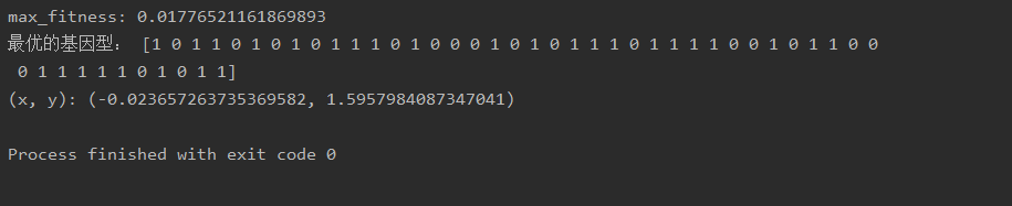
print("max_fitness:", fitness[max_fitness_index])
x, y = translateDNA(pop)
print("最优的基因型:", pop[max_fitness_index])
print("(x, y):", (x[max_fitness_index], y[max_fitness_index]))
if __name__ == "__main__":
fig = plt.figure()
ax = Axes3D(fig)
plt.ion() # 将画图模式改为交互模式,程序遇到plt.show不会暂停,而是继续执行
plot_3d(ax)
pop = np.random.randint(2, size=(POP_SIZE, DNA_SIZE * 2)) # matrix (POP_SIZE, DNA_SIZE)
for _ in range(N_GENERATIONS): # 迭代N代
x, y = translateDNA(pop)
if 'sca' in locals():
sca.remove()
sca = ax.scatter(x, y, F(x, y), c='black', marker='o');
plt.show()
plt.pause(0.1)
pop = np.array(crossover_and_mutation(pop, CROSSOVER_RATE))
# F_values = F(translateDNA(pop)[0], translateDNA(pop)[1])#x, y --> Z matrix
fitness = get_fitness(pop)
pop = select(pop, fitness) # 选择生成新的种群
print_info(pop)
plt.ioff()
plot_3d(ax)
统计分析模型
Logistic回归(逻辑回归)
如果觉得这个代码过多,可以使用sklearn中的LogisticRegression。具体如何调用在下一个代码。
import numpy as np
import pandas as pd
import numpy.random
import matplotlib.pyplot as plt
import time
import os
from sklearn import preprocessing as pp

# 导入数据
path = 'data' + os.sep + 'Logireg_data.txt'
pdData = pd.read_csv(path, header=None, names=['Exam1', 'Exam2', 'Admitted'])
pdData.head()
print(pdData.head())
print(pdData.shape)
positive = pdData[pdData['Admitted'] == 1]  # 定义正
nagative = pdData[pdData['Admitted'] == 0]  # 定义负
fig, ax = plt.subplots(figsize=(10, 5))
ax.scatter(positive['Exam1'], positive['Exam2'], s=30, c='b', marker='o', label='Admitted')
ax.scatter(nagative['Exam1'], nagative['Exam2'], s=30, c='r', marker='x', label='not Admitted')
ax.legend()
ax.set_xlabel('Exam 1 score')
ax.set_ylabel('Exam 2 score')
plt.show()  # 画图


# 实现算法 the logistics regression 目标建立一个分类器 设置阈值来判断录取结果
# sigmoid 函数
def sigmoid(z):
    return 1 / (1 + np.exp(-z))


# 画图
nums = np.arange(-10, 10, step=1)
fig, ax = plt.subplots(figsize=(12, 4))
ax.plot(nums, sigmoid(nums), 'r')  # 画图定义
plt.show()


# 按照理论实现预测函数
def model(X, theta):
    return sigmoid(np.dot(X, theta.T))


pdData.insert(0, 'ones', 1)  # 插入一列
orig_data=pdData.as_matrix()
cols=orig_data.shape[1]
X=orig_data[:, 0:cols - 1]
y=orig_data[:, cols - 1:cols]
theta=np.zeros([1, 3])
print(X[:5])
print(X.shape, y.shape, theta.shape)


# 损失函数
def cost(X, y, theta):
    left=np.multiply(-y, np.log(model(X, theta)))
    right=np.multiply(1 - y, np.log(1 - model(X, theta)))
    return np.sum(left - right) / (len(X))


print(cost(X, y, theta))


# 计算梯度
def gradient(X, y, theta):
    grad=np.zeros(theta.shape)
    error=(model(X, theta) - y).ravel()
    for j in range(len(theta.ravel())):  # for each parmeter
        term=np.multiply(error, X[:, j])
        grad[0, j]=np.sum(term) / len(X)

    return grad


# 比较3种不同梯度下降方法
STOP_ITER = 0
STOP_COST = 1
STOP_GRAD = 2


def stopCriterion(type, value, threshold):
    if type == STOP_ITER:
        return value > threshold
    elif type == STOP_COST:
        return abs(value[-1] - value[-2]) < threshold
    elif type == STOP_GRAD:
        return np.linalg.norm(value) < threshold


# 打乱数据洗牌
def shuffledata(data):
    np.random.shuffle(data)
    cols = data.shape[1]
    X = data[:, 0:cols - 1]
    y = data[:, cols - 1:]
    return X, y


def descent(data, theta, batchSize, stopType, thresh, alpha):
    # 梯度下降求解

    init_time = time.time()
    i = 0  # 迭代次数
    k = 0  # batch
    X, y = shuffledata(data)
    grad = np.zeros(theta.shape)  # 计算的梯度
    costs = [cost(X, y, theta)]  # 损失值

    while True:
        grad = gradient(X[k:k + batchSize], y[k:k + batchSize], theta)
        k += batchSize  # 取batch数量个数据
        if k >= n:
            k = 0
            X, y = shuffledata(data)  # 重新洗牌
        theta = theta - alpha * grad  # 参数更新
        costs.append(cost(X, y, theta))  # 计算新的损失
        i += 1

        if stopType == STOP_ITER:
            value = i
        elif stopType == STOP_COST:
            value = costs
        elif stopType == STOP_GRAD:
            value = grad
        if stopCriterion(stopType, value, thresh): break

    return theta, i - 1, costs, grad, time.time() - init_time


# 选择梯度下降
def runExpe(data, theta, batchSize, stopType, thresh, alpha):
    # import pdb; pdb.set_trace();
    theta, iter, costs, grad, dur=descent(data, theta, batchSize, stopType, thresh, alpha)
    name = "Original" if (data[:, 1] > 2).sum() > 1 else "Scaled"
    name += " data - learning rate: {} - ".format(alpha)
    if batchSize == n:
        strDescType="Gradient"
    elif batchSize == 1:
        strDescType = "Stochastic"
    else:
        strDescType = "Mini-batch ({})".format(batchSize)
    name += strDescType + " descent - Stop: "
    if stopType == STOP_ITER:
        strStop = "{} iterations".format(thresh)
    elif stopType == STOP_COST:
        strStop = "costs change < {}".format(thresh)
    else:
        strStop = "gradient norm < {}".format(thresh)
    name += strStop
    print("***{}\nTheta: {} - Iter: {} - Last cost: {:03.2f} - Duration: {:03.2f}s".format(
        name, theta, iter, costs[-1], dur))
    fig, ax = plt.subplots(figsize=(12, 4))
    ax.plot(np.arange(len(costs)), costs, 'r')
    ax.set_xlabel('Iterations')
    ax.set_ylabel('Cost')
    ax.set_title(name.upper() + ' - Error vs. Iteration')
    return theta


n = 100
runExpe(orig_data, theta, n, STOP_ITER, thresh=5000, alpha=0.000001)
plt.show()
runExpe(orig_data, theta, n, STOP_GRAD, thresh=0.05, alpha=0.001)
plt.show()
runExpe(orig_data, theta, n, STOP_COST, thresh=0.000001, alpha=0.001)
plt.show()
# 对比
runExpe(orig_data, theta, 1, STOP_ITER, thresh=5000, alpha=0.001)
plt.show()
runExpe(orig_data, theta, 1, STOP_ITER, thresh=15000, alpha=0.000002)
plt.show()
runExpe(orig_data, theta, 16, STOP_ITER, thresh=15000, alpha=0.001)
plt.show()
# 对数据进行标准化 将数据按其属性(按列进行)减去其均值,然后除以其方差。
# 最后得到的结果是,对每个属性/每列来说所有数据都聚集在0附近,方差值为1


scaled_data = orig_data.copy()
scaled_data[:, 1:3] = pp.scale(orig_data[:, 1:3])

runExpe(scaled_data, theta, n, STOP_ITER, thresh=5000, alpha=0.001)


# 设定阈值
def predict(X, theta):
    return [1 if x >= 0.5 else 0 for x in model(X, theta)]


scaled_X = scaled_data[:, :3]
y = scaled_data[:, 3]
predictions = predict(scaled_X, theta)
correct = [1 if ((a == 1 and b == 1) or (a == 0 and b == 0)) else 0 for (a, b) in zip(predictions, y)]
accuracy = (sum(map(int, correct)) % len(correct))
print('accuracy = {0}%'.format(accuracy))
from sklearn.linear_model import LogisticRegression

XTrain = [[0, 0], [1, 1]]
YTrain = [0, 1]
reg = LogisticRegression()
reg.fit(XTrain, YTrain)
print(reg.score(XTrain, YTrain))
具体参数的详解和使用可以看下这篇知乎文章文章地址
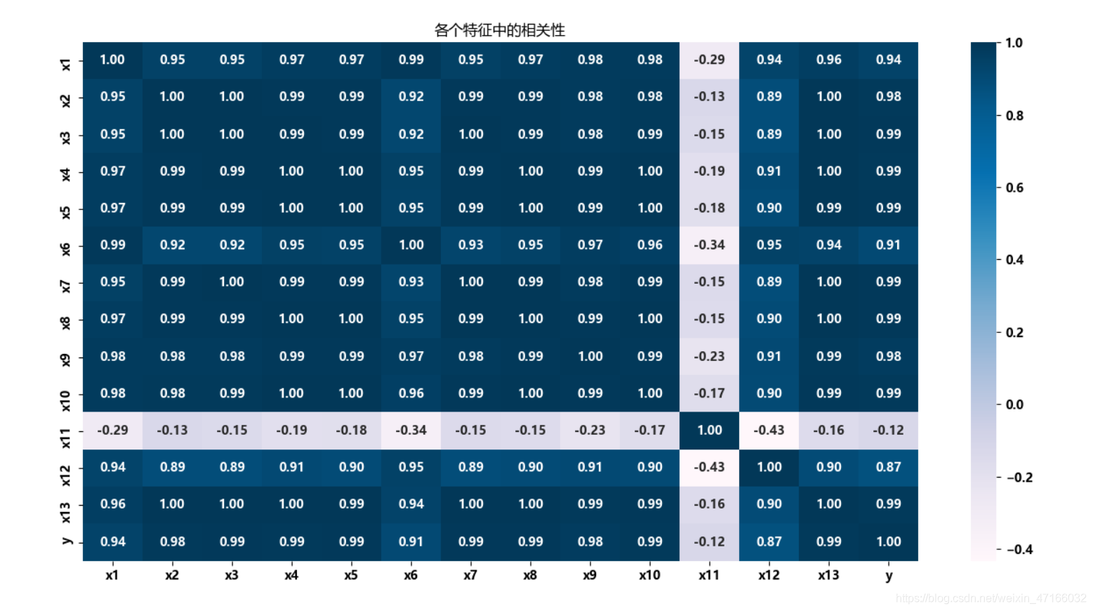
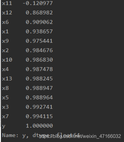
相关性分析
import matplotlib.pyplot as plt
import pandas as pd
import seaborn as sns


# 导入数据
data = pd.read_csv(r'C:\data.csv')
x_data = data.drop('y', 1)
y_data = data.loc[:, 'y']
name_data = list(data.columns.values)
warnings.filterwarnings("ignore")  # 排除警告信息
plt.figure(figsize=(12, 8))
sns.heatmap(data.corr(), annot=True, fmt='.2f', cmap='PuBu')
plt.title('各个特征中的相关性')
plt.show()
# 打印Pearson相关系数
print(data.corr()['y'].sort_values())
主成分分析(PCA)
import matplotlib.pyplot as plt
from sklearn.decomposition import PCA
from sklearn.datasets import load_iris

data = load_iris()
y = data.target
x = data.data
pca = PCA(n_components=2)  # 加载PCA算法,设置降维后主成分数目为2
reduced_x = pca.fit_transform(x)  # 对样本进行降维
red_x, red_y = [], []
blue_x, blue_y = [], []
green_x, green_y = [], []

for i in range(len(reduced_x)):
    if y[i] == 0:
        red_x.append(reduced_x[i][0])
        red_y.append(reduced_x[i][1])
    elif y[i] == 1:
        blue_x.append(reduced_x[i][0])
        blue_y.append(reduced_x[i][1])
    else:
        green_x.append(reduced_x[i][0])
        green_y.append(reduced_x[i][1])
# 可视化
plt.scatter(red_x, red_y, c='r', marker='x')
plt.scatter(blue_x, blue_y, c='b', marker='D')
plt.scatter(green_x, green_y, c='g', marker='.')
plt.show()
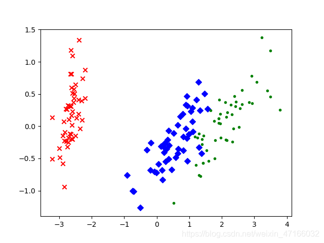
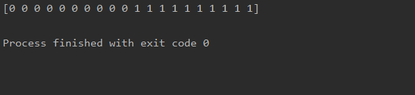
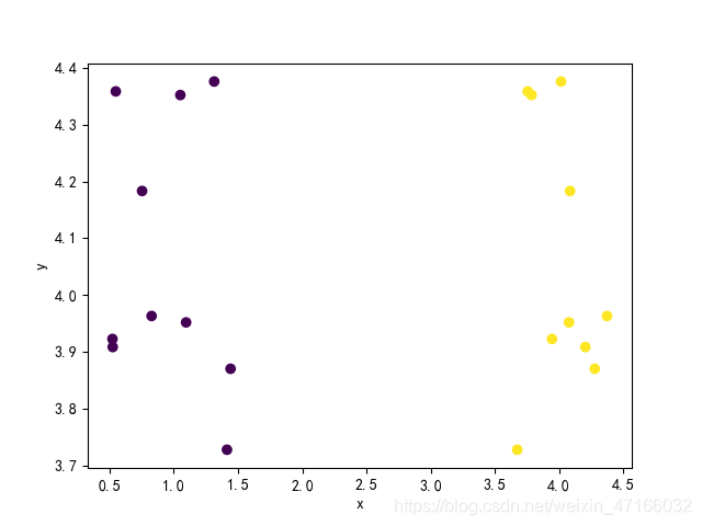
聚类分析
import matplotlib.pyplot as plt
from sklearn.cluster import KMeans
from scipy.spatial.distance import cdist
import numpy as np
# 创建训练数据,建模比赛时可以直接导入数据文件
c1x = np.random.uniform(0.5, 1.5, (1, 10))
c1y = np.random.uniform(0.5, 1.5, (1, 10))
c2x = np.random.uniform(3.5, 4.5, (1, 10))
c2y = np.random.uniform(3.5, 4.5, (1, 10))
x = np.hstack((c1x, c2x))
y = np.hstack((c2y, c2y))
X = np.vstack((x, y)).T
# 导入模型
kemans = KMeans(n_clusters=2)
result = kemans.fit_predict(X) # 训练及预测
print(result) # 分类结果
plt.rcParams['font.family'] = ['sans-serif']
plt.rcParams['font.sans-serif'] = ['SimHei'] # 散点图标签可以显示中文
x = [i[0] for i in X]
y = [i[1] for i in X]
plt.scatter(x, y, c=result, marker='o')
plt.xlabel('x')
plt.ylabel('y')
plt.show()
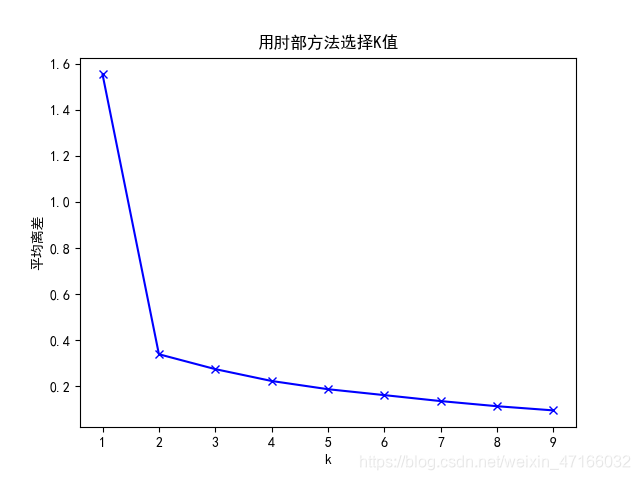
# 如果K值未知,可采用肘部法选择K值
K = range(1, 10)
meanDispersions = []
for k in K:
kemans = KMeans(n_clusters=k)
kemans.fit(X)
# 计算平均离差
m_Disp = sum(np.min(cdist(X, kemans.cluster_centers_, 'euclidean'), axis=1)) / X.shape[0]
meanDispersions.append(m_Disp)
plt.plot(K, meanDispersions, 'bx-')
plt.xlabel('k')
plt.ylabel('平均离差')
plt.title('用肘部方法选择K值')
plt.show()
动态模型
微分方程模型
以下微分方程模型代码来自博主youcans的文章:https://blog.csdn.net/youcans/article/details/117702996
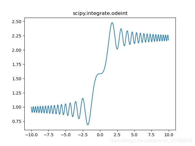
一阶常微分方程
# 1. 求解微分方程初值问题(scipy.integrate.odeint)
from scipy.integrate import odeint
import numpy as np
import matplotlib.pyplot as plt


def dy_dt(y, t):  # 定义函数 f(y,t)
    return np.sin(t**2)


y0 = [1]  # y0 = 1 也可以
t = np.arange(-10, 10, 0.01)  # (start,stop,step)
y = odeint(dy_dt, y0, t)  # 求解微分方程初值问题

# 绘图
plt.plot(t, y)
plt.title("scipy.integrate.odeint")
plt.show()
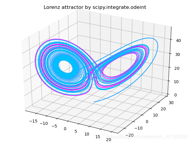
一阶常微分方程组
# 2. 求解微分方程组初值问题(scipy.integrate.odeint)
from scipy.integrate import odeint
import numpy as np
import matplotlib.pyplot as plt
from mpl_toolkits.mplot3d import Axes3D


# 导数函数, 求 W=[x,y,z] 点的导数 dW/dt
def lorenz(W,t,p,r,b):  # by youcans
    x, y, z = W  # W=[x,y,z]
    dx_dt = p*(y-x)  # dx/dt = p*(y-x), p: sigma
    dy_dt = x*(r-z) - y  # dy/dt = x*(r-z)-y, r:rho
    dz_dt = x*y - b*z  # dz/dt = x*y - b*z, b;beta
    return np.array([dx_dt,dy_dt,dz_dt])


t = np.arange(0, 30, 0.01)  # 创建时间点 (start,stop,step)
paras = (10.0, 28.0, 3.0)  # 设置 Lorenz 方程中的参数 (p,r,b)

# 调用ode对lorenz进行求解, 用两个不同的初始值 W1、W2 分别求解
W1 = (0.0, 1.00, 0.0)  # 定义初值为 W1
track1 = odeint(lorenz, W1, t, args=(10.0, 28.0, 3.0))  # args 设置导数函数的参数
W2 = (0.0, 1.01, 0.0)  # 定义初值为 W2
track2 = odeint(lorenz, W2, t, args=paras)  # 通过 paras 传递导数函数的参数

# 绘图
fig = plt.figure()
ax = Axes3D(fig)
ax.plot(track1[:, 0], track1[:, 1], track1[:, 2], color='magenta')  # 绘制轨迹 1
ax.plot(track2[:, 0], track2[:, 1], track2[:, 2], color='deepskyblue')  # 绘制轨迹 2
ax.set_title("Lorenz attractor by scipy.integrate.odeint")
plt.show()
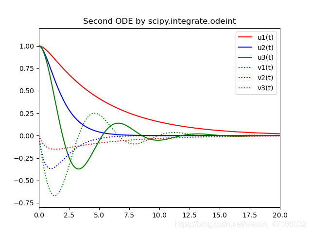
二阶微分方程
# 3. 求解二阶微分方程初值问题(scipy.integrate.odeint)
# Second ODE by scipy.integrate.odeint
from scipy.integrate import odeint
import numpy as np
import matplotlib.pyplot as plt


# 导数函数,求 Y=[u,v] 点的导数 dY/dt
def deriv(Y, t, a, w):
    u, v = Y  # Y=[u,v]
    dY_dt = [v, -2*a*v-w*w*u]
    return dY_dt


t = np.arange(0, 20, 0.01)  # 创建时间点 (start,stop,step)
# 设置导数函数中的参数 (a, w)
paras1 = (1, 0.6)  # 过阻尼:a^2 - w^2 > 0
paras2 = (1, 1)  # 临界阻尼:a^2 - w^2 = 0
paras3 = (0.3, 1)  # 欠阻尼:a^2 - w^2 < 0

# 调用ode对进行求解, 用两个不同的初始值 W1、W2 分别求解
Y0 = (1.0, 0.0)  # 定义初值为 Y0=[u0,v0]
Y1 = odeint(deriv, Y0, t, args=paras1)  # args 设置导数函数的参数
Y2 = odeint(deriv, Y0, t, args=paras2)  # args 设置导数函数的参数
Y3 = odeint(deriv, Y0, t, args=paras3)  # args 设置导数函数的参数
# W2 = (0.0, 1.01, 0.0)  # 定义初值为 W2
# track2 = odeint(lorenz, W2, t, args=paras)  # 通过 paras 传递导数函数的参数

# 绘图
plt.plot(t, Y1[:, 0], 'r-', label='u1(t)')
plt.plot(t, Y2[:, 0], 'b-', label='u2(t)')
plt.plot(t, Y3[:, 0], 'g-', label='u3(t)')
plt.plot(t, Y1[:, 1], 'r:', label='v1(t)')
plt.plot(t, Y2[:, 1], 'b:', label='v2(t)')
plt.plot(t, Y3[:, 1], 'g:', label='v3(t)')
plt.axis([0, 20, -0.8, 1.2])
plt.legend(loc='best')
plt.title("Second ODE by scipy.integrate.odeint")
plt.show()
其他一些常用模型
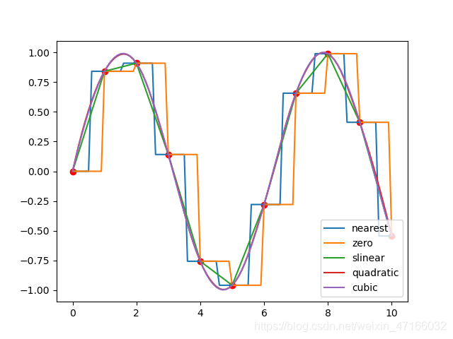
一维差值
# -*-coding:utf-8 -*-
import numpy as np
from scipy import interpolate
import pylab as pl

x = np.linspace(0,10,11)
#x=[  0.   1.   2.   3.   4.   5.   6.   7.   8.   9.  10.]
y = np.sin(x)
xnew = np.linspace(0, 10, 101)
pl.plot(x, y, "ro")

for kind in ["nearest", "zero", "slinear", "quadratic", "cubic"]:  # 插值方式
    #"nearest","zero"为阶梯插值
    #slinear 线性插值
    #"quadratic","cubic" 为2阶、3阶B样条曲线插值
    f = interpolate.interp1d(x,y,kind=kind)
    # ‘slinear’, ‘quadratic’ and ‘cubic’ refer to a spline interpolation of first, second or third order)
    ynew = f(xnew)
    pl.plot(xnew, ynew, label=str(kind))
pl.legend(loc="lower right")
pl.show()
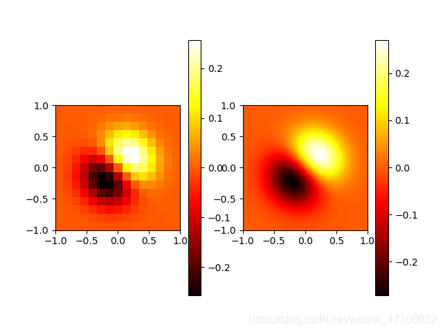
二维插值
import numpy as np
from scipy import interpolate
import pylab as pl
import matplotlib as mpl


def func(x, y):
    return (x+y)*np.exp(-5.0*(x**2 + y**2))


# X-Y轴分为15*15的网格
y, x = np.mgrid[-1:1:15j, -1:1:15j]

fvals = func(x, y)  # 计算每个网格点上的函数值  15*15的值
print(len(fvals[0]))

# 三次样条二维插值
newfunc = interpolate.interp2d(x, y, fvals, kind='cubic')

# 计算100*100的网格上的插值
xnew = np.linspace(-1, 1, 100)  # x
ynew = np.linspace(-1, 1, 100)  # y
fnew = newfunc(xnew, ynew)  # 仅仅是y值   100*100的值

# 绘图
# 为了更明显地比较插值前后的区别,使用关键字参数interpolation='nearest'
# 关闭imshow()内置的插值运算。
pl.subplot(121)
im1 = pl.imshow(fvals, extent=[-1, 1, -1, 1], cmap=mpl.cm.hot, interpolation='nearest', origin="lower")  # pl.cm.jet
# extent=[-1,1,-1,1]为x,y范围  favals为
pl.colorbar(im1)

pl.subplot(122)
im2 = pl.imshow(fnew, extent=[-1, 1, -1, 1], cmap=mpl.cm.hot, interpolation='nearest', origin="lower")
pl.colorbar(im2)
pl.show()
BP神经网络模型
# -*- coding: utf-8 -*-
# 参考https://blog.csdn.net/jiangjiang_jian/article/details/79031788
import numpy as np
import math
import random
import string
import matplotlib as mpl
import matplotlib.pyplot as plt


# random.seed(0)  #当我们设置相同的seed,每次生成的随机数相同。如果不设置seed,则每次会生成不同的随机数
# 生成区间[a,b]内的随机数
def random_number(a, b):
    return (b - a) * random.random() + a


# 生成一个矩阵,大小为m*n,并且设置默认零矩阵
def makematrix(m, n, fill=0.0):
    a = []
    for i in range(m):
        a.append([fill] * n)
    return a


# 函数sigmoid(),这里采用tanh,因为看起来要比标准的sigmoid函数好看
def sigmoid(x):
    return math.tanh(x)


# 函数sigmoid的派生函数
def derived_sigmoid(x):
    return 1.0 - x ** 2


# 构造三层BP网络架构
class BPNN:
    def __init__(self, num_in, num_hidden, num_out):
        # 输入层,隐藏层,输出层的节点数
        self.num_in = num_in + 1  # 增加一个偏置结点
        self.num_hidden = num_hidden + 1  # 增加一个偏置结点
        self.num_out = num_out

        # 激活神经网络的所有节点(向量)
        self.active_in = [1.0] * self.num_in
        self.active_hidden = [1.0] * self.num_hidden
        self.active_out = [1.0] * self.num_out

        # 创建权重矩阵
        self.wight_in = makematrix(self.num_in, self.num_hidden)
        self.wight_out = makematrix(self.num_hidden, self.num_out)

        # 对权值矩阵赋初值
        for i in range(self.num_in):
            for j in range(self.num_hidden):
                self.wight_in[i][j] = random_number(-0.2, 0.2)
        for i in range(self.num_hidden):
            for j in range(self.num_out):
                self.wight_out[i][j] = random_number(-0.2, 0.2)

        # 最后建立动量因子(矩阵)
        self.ci = makematrix(self.num_in, self.num_hidden)
        self.co = makematrix(self.num_hidden, self.num_out)

        # 信号正向传播

    def update(self, inputs):
        if len(inputs) != self.num_in - 1:
            raise ValueError('与输入层节点数不符')

        # 数据输入输入层
        for i in range(self.num_in - 1):
            # self.active_in[i] = sigmoid(inputs[i])  #或者先在输入层进行数据处理
            self.active_in[i] = inputs[i]  # active_in[]是输入数据的矩阵

        # 数据在隐藏层的处理
        for i in range(self.num_hidden - 1):
            sum = 0.0
            for j in range(self.num_in):
                sum = sum + self.active_in[i] * self.wight_in[j][i]
            self.active_hidden[i] = sigmoid(sum)  # active_hidden[]是处理完输入数据之后存储,作为输出层的输入数据

        # 数据在输出层的处理
        for i in range(self.num_out):
            sum = 0.0
            for j in range(self.num_hidden):
                sum = sum + self.active_hidden[j] * self.wight_out[j][i]
            self.active_out[i] = sigmoid(sum)  # 与上同理

        return self.active_out[:]

    # 误差反向传播
    def errorbackpropagate(self, targets, lr, m):  # lr是学习率, m是动量因子
        if len(targets) != self.num_out:
            raise ValueError('与输出层节点数不符!')

        # 首先计算输出层的误差
        out_deltas = [0.0] * self.num_out
        for i in range(self.num_out):
            error = targets[i] - self.active_out[i]
            out_deltas[i] = derived_sigmoid(self.active_out[i]) * error

        # 然后计算隐藏层误差
        hidden_deltas = [0.0] * self.num_hidden
        for i in range(self.num_hidden):
            error = 0.0
            for j in range(self.num_out):
                error = error + out_deltas[j] * self.wight_out[i][j]
            hidden_deltas[i] = derived_sigmoid(self.active_hidden[i]) * error

        # 首先更新输出层权值
        for i in range(self.num_hidden):
            for j in range(self.num_out):
                change = out_deltas[j] * self.active_hidden[i]
                self.wight_out[i][j] = self.wight_out[i][j] + lr * change + m * self.co[i][j]
                self.co[i][j] = change

        # 然后更新输入层权值
        for i in range(self.num_in):
            for i in range(self.num_hidden):
                change = hidden_deltas[j] * self.active_in[i]
                self.wight_in[i][j] = self.wight_in[i][j] + lr * change + m * self.ci[i][j]
                self.ci[i][j] = change

        # 计算总误差
        error = 0.0
        for i in range(len(targets)):
            error = error + 0.5 * (targets[i] - self.active_out[i]) ** 2
        return error

    # 测试
    def test(self, patterns):
        for i in patterns:
            print(i[0], '->', self.update(i[0]))

    # 权重
    def weights(self):
        print("输入层权重")
        for i in range(self.num_in):
            print(self.wight_in[i])
        print("输出层权重")
        for i in range(self.num_hidden):
            print(self.wight_out[i])

    def train(self, pattern, itera=100000, lr=0.1, m=0.1):
        for i in range(itera):
            error=0.0
            for j in pattern:
                inputs = j[0]
                targets = j[1]
                self.update(inputs)
                error = error + self.errorbackpropagate(targets, lr, m)
            if i % 100 == 0:
                print('误差 %-.5f' % error)


# 实例
def demo():
    patt = [
        [[1, 2, 5], [0]],
        [[1, 3, 4], [1]],
        [[1, 6, 2], [1]],
        [[1, 5, 1], [0]],
        [[1, 8, 4], [1]]
    ]
    # 创建神经网络,3个输入节点,3个隐藏层节点,1个输出层节点
    n = BPNN(3, 3, 1)
    # 训练神经网络
    n.train(patt)
    # 测试神经网络
    n.test(patt)
    # 查阅权重值
    n.weights()


if __name__ == '__main__':
    demo()
总结
以上代码为总结性代码,有些复制了部分博主的代码和书本上的代码,如有侵权,请告知删除。为什么要总结这些代码,其实学习数学建模来说,很多同学对其模型或者算法的理论都了解,但难以使用代码实践,或者不熟悉matlab,所以总结了这些常用模型的python代码。一次建模,终身受益,愿与各位同学共同进步。