声明
声明:未经允许,不得转载。——CSDN:川川菜鸟
数学虽然有些难度,当时我们如果把它们转化为容易看懂的,就如此简单。这些函数和代码是我最近几天在做寻优算法的时候总结的,因此本篇内容主要是展示可视化部分,并没有谈到任何算法。
前半部分我给了具体公式,后面部分我实在懒得弄公式了,主要是带大家感受数学的优美,不要对数学感到困难情绪。
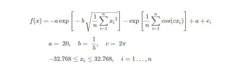
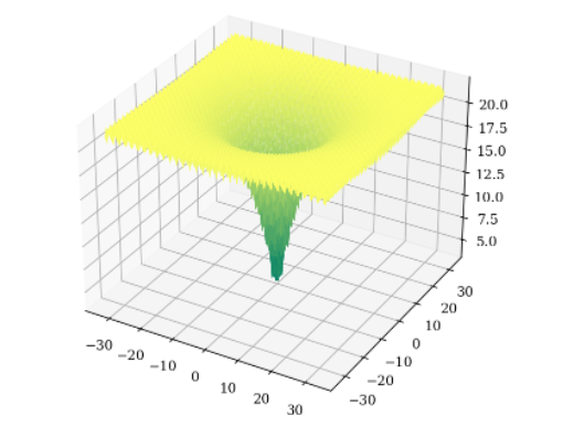
Ackley函数
公式如下:
代码编写:
import numpy as np

from pymoo.problems import get_problem
from pymoo.visualization.fitness_landscape import FitnessLandscape

problem = get_problem("ackley", n_var=2, a=20, b=1/5, c=2 * np.pi)

FitnessLandscape(problem, angle=(45, 45), _type="surface").show()
绘制函数图形如下:
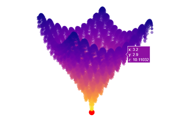
换个画法:
from pyMetaheuristic.test_function import single
from pyMetaheuristic.utils import graphs

tf = single.ackley

# Target Function - 3D Plot
plot_parameters = {


    'min_values': (-5, -5),
    'max_values': (5, 5),
    'step': (0.1, 0.1),
    'solution': [(0, 0)],
    'proj_view': '3D',
    'view': 'notebook'
}
graphs.plot_single_function(target_function = tf, **plot_parameters)
如下:
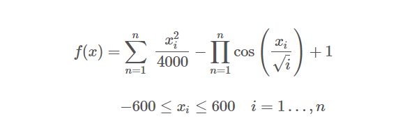
Griewank函数
公式如下:
代码编写:
from pymoo.problems import get_problem
from pymoo.visualization.fitness_landscape import FitnessLandscape

problem = get_problem("griewank", n_var=1)
plot = FitnessLandscape(problem, _type="surface", n_samples=1000)
plot.do()
plot.apply(lambda ax: ax.set_xlim(-200, 200))
plot.apply(lambda ax: ax.set_ylim(-1, 13))
plot.show()
绘制如下:

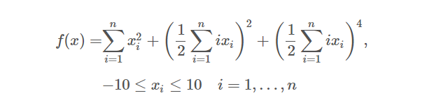
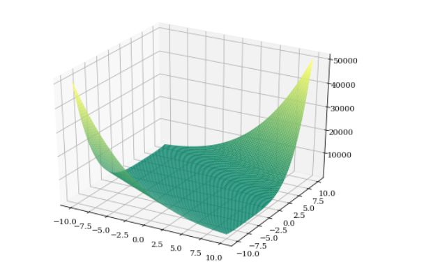
Zakharov函数
公式如下:
代码编写:
import numpy as np

from pymoo.problems import get_problem
from pymoo.visualization.fitness_landscape import FitnessLandscape

problem = get_problem("zakharov", n_var=2)

FitnessLandscape(problem, angle=(45, 45), _type="surface").show()
绘制如下:
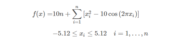
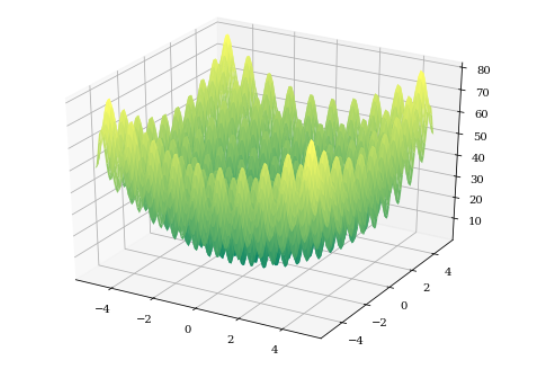
rastrigin函数
公式如下:
代码如下:
import numpy as np

from pymoo.problems import get_problem
from pymoo.visualization.fitness_landscape import FitnessLandscape

problem = get_problem("rastrigin", n_var=2)

FitnessLandscape(problem, angle=(45, 45), _type="surface").show()
绘制如下:
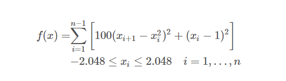
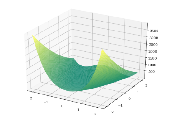
Rosenbrock函数
公式如下:
代码编写:
import numpy as np

from pymoo.problems import get_problem
from pymoo.visualization.fitness_landscape import FitnessLandscape

problem = get_problem("rosenbrock", n_var=2)

FitnessLandscape(problem, angle=(45, 45), _type="surface").show()
绘制如下:
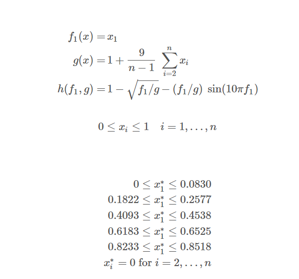
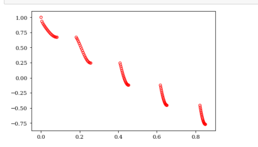
ZDT3函数
公式如下:
代码编写:
from pymoo.problems import get_problem
from pymoo.util.plotting import plot

problem = get_problem("zdt3")
plot(problem.pareto_front(), no_fill=True)
如下:
TNK函数
公式如下:
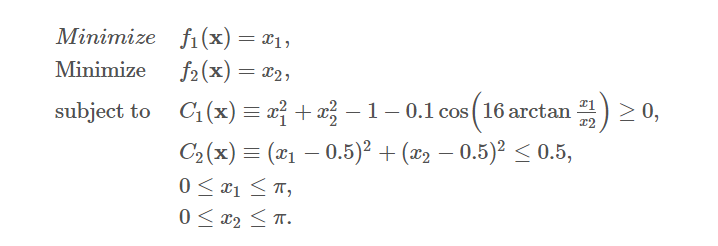
代码编写:
from pymoo.problems import get_problem
from pymoo.util.plotting import plot

problem = get_problem("tnk")
plot(problem.pareto_front(), no_fill=True)
如下:
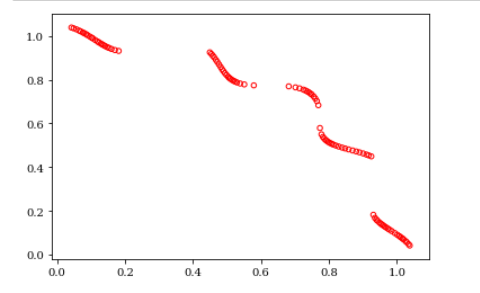
DF3函数
代码如下:
from pymoo.problems.dynamic.df import DF3

plot = Scatter()

for t in np.linspace(0, 10.0, 100):
    problem = DF3(time=t)
    plot.add(problem.pareto_front(), plot_type="line", color="black", alpha=0.7)

plot.show()
绘制如下:
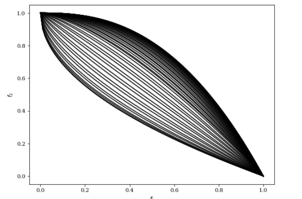
DF4函数
from pymoo.problems.dynamic.df import DF4

plot = Scatter()

for t in np.linspace(0, 10.0, 100):
    problem = DF4(time=t)
    plot.add(problem.pareto_front() + 2*t, plot_type="line", color="black", alpha=0.7)

plot.show()
如下:
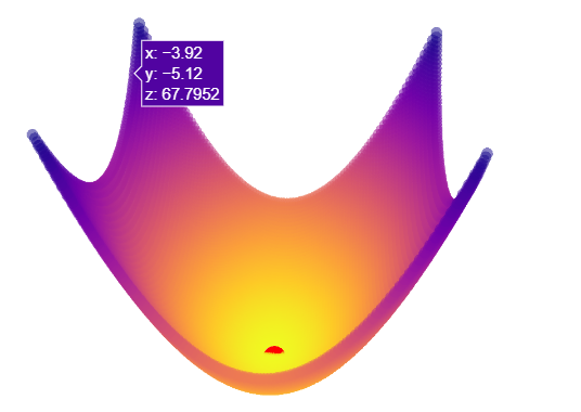
arallel_hyper_ellipsoid 函数
tf = single.axis_parallel_hyper_ellipsoid


plot_parameters = {


    'min_values': (-5.12, -5.12),
    'max_values': (5.12, 5.12),
    'step': (0.1, 0.1),
    'solution': [(0, 0)],
    'proj_view': '3D',
    'view': 'notebook'
}
graphs.plot_single_function(target_function = tf, **plot_parameters)
如下:
beale函数
tf = single.beale

plot_parameters = {


    'min_values': (-4.5, -4.52),
    'max_values': (4,5, 4.5),
    'step': (0.1, 0.1),
    'solution': [(3, 0.5)],
    'proj_view': '3D',
    'view': 'notebook'
}
graphs.plot_single_function(target_function = tf, **plot_parameters)
如下:
booth函数
tf = single.booth


plot_parameters = {


    'min_values': (-10, -10),
    'max_values': (10, 10),
    'step': (0.1, 0.1),
    'solution': [(1, 3)],
    'proj_view': '3D',
    'view': 'notebook'
}
graphs.plot_single_function(target_function = tf, **plot_parameters)
如下:
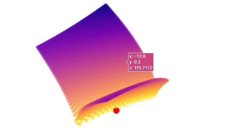
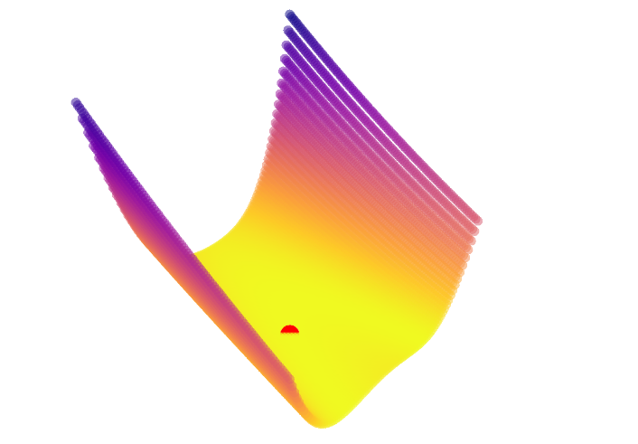
branin_rcos函数
tf = single.branin_rcos


plot_parameters = {


    'min_values': (-5, 0),
    'max_values': (10, 15),
    'step': (0.1, 0.1),
    'solution': [(-3.14, 12.275), (3.14, 2.275), (9.42478, 2.475)],
    'proj_view': '3D',
    'view': 'notebook'
}
graphs.plot_single_function(target_function = tf, **plot_parameters)
如下:
bukin_6函数
tf = single.bukin_6


plot_parameters = {


    'min_values': (-15, -3),
    'max_values': (-5, 3),
    'step': (0.1, 0.1),
    'solution': [(-10, 1)],
    'proj_view': '3D',
    'view': 'notebook'
}
graphs.plot_single_function(target_function = tf, **plot_parameters)
绘制如下:
Cross in Tray函数
tf = single.cross_in_tray


plot_parameters = {


    'min_values': (-10, -10),
    'max_values': (10, 10),
    'step': (0.1, 0.1),
    'solution': [(1.34941, 1.34941), (-1.34941, 1.34941), (1.34941, -1.34941), (-1.34941, -1.34941)],
    'proj_view': '3D',
    'view': 'notebook'
}
graphs.plot_single_function(target_function = tf, **plot_parameters)
绘制如下:
de_jong_1函数
tf = single.de_jong_1


plot_parameters = {


    'min_values': (-5.12, -5.12),
    'max_values': (5.12, 5.12),
    'step': (0.1, 0.1),
    'solution': [(0, 0)],
    'proj_view': '3D',
    'view': 'notebook'
}
graphs.plot_single_function(target_function = tf, **plot_parameters)
如下:

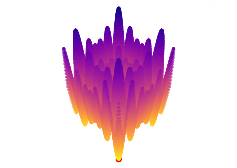
drop_wave函数
tf = single.drop_wave

plot_parameters = {


    'min_values': (-5.12, -5.12),
    'max_values': (5.12, 5.12),
    'step': (0.1, 0.1),
    'solution': [(0, 0)],
    'proj_view': '3D',
    'view': 'notebook'
}
graphs.plot_single_function(target_function = tf, **plot_parameters)
如下:
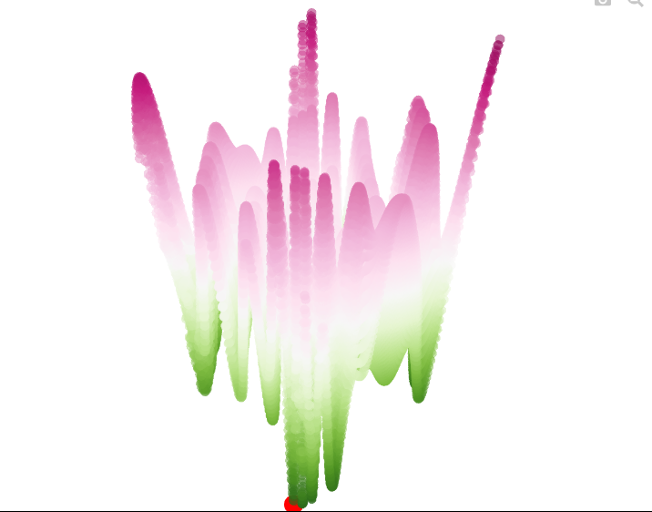
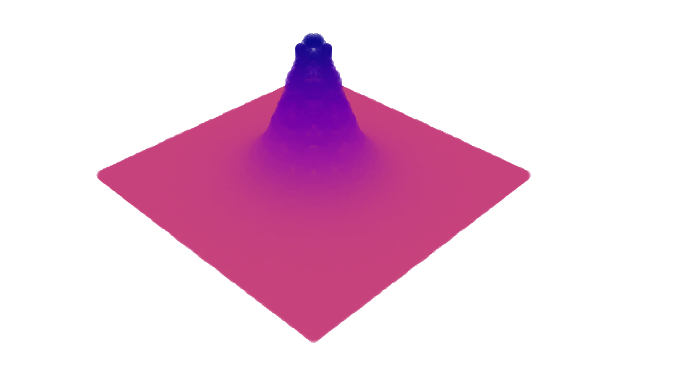
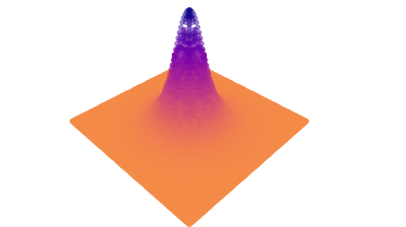
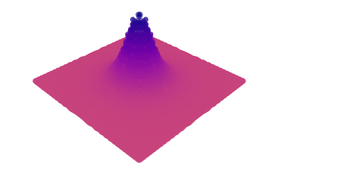
easom函数
tf = single.easom

plot_parameters = {


    'min_values': (-100, -100),
    'max_values': (100, 100),
    'step': (1, 1),
    'solution': [(3.14, 3.14)],
    'proj_view': '3D',
    'view': 'notebook'
}
graphs.plot_single_function(target_function = tf, **plot_parameters)
如下:
eggholder函数
tf = single.eggholder


plot_parameters = {


    'min_values': (-512, -512),
    'max_values': (512, 512),
    'step': (5, 5),
    'solution': [(512, 404.2319)],
    'proj_view': '3D',
    'view': 'notebook'
}
graphs.plot_single_function(target_function = tf, **plot_parameters)
绘制如下:
goldstein_price函数
tf = single.goldstein_price


plot_parameters = {


    'min_values': (-2, -2),
    'max_values': (2, 2),
    'step': (0.05, 0.05),
    'solution': [(0, -1)],
    'proj_view': '3D',
    'view': 'notebook'
}
graphs.plot_single_function(target_function = tf, **plot_parameters)
绘制如下:
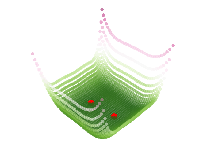
himmelblau函数
tf = single.himmelblau


plot_parameters = {


    'min_values': (-5, -5),
    'max_values': (5, 5),
    'step': (0.1, 0.1),
    'solution': [(3, 2), (-2.805118, 3.131312), (-3.779310, -3.283186), (3.584428 ,-1.848126)],
    'proj_view': '3D',
    'view': 'notebook'
}
graphs.plot_single_function(target_function = tf, **plot_parameters)
如下:
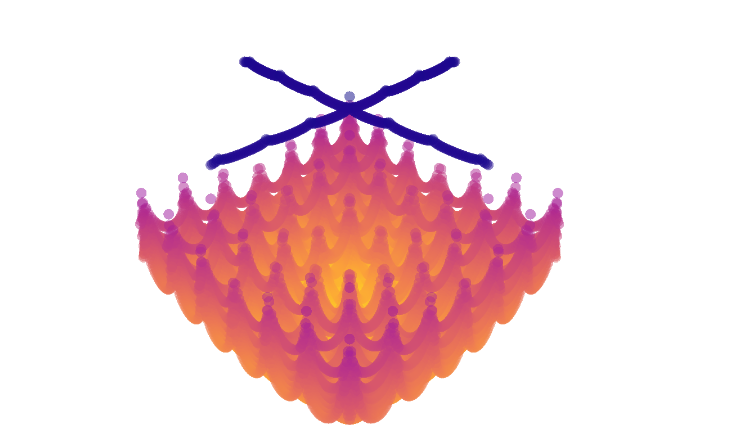
holder_table函数
tf = single.holder_table


plot_parameters = {


    'min_values': (-10, -10),
    'max_values': (10, 10),
    'step': (0.1, 0.1),
    'solution': [(8.05502, 9.66459), (-8.05502, 9.66459), (8.05502, -9.66459), (-8.05502, -9.66459)],
    'proj_view': '3D',
    'view': 'notebook'
}
graphs.plot_single_function(target_function = tf, **plot_parameters)
绘制如下:
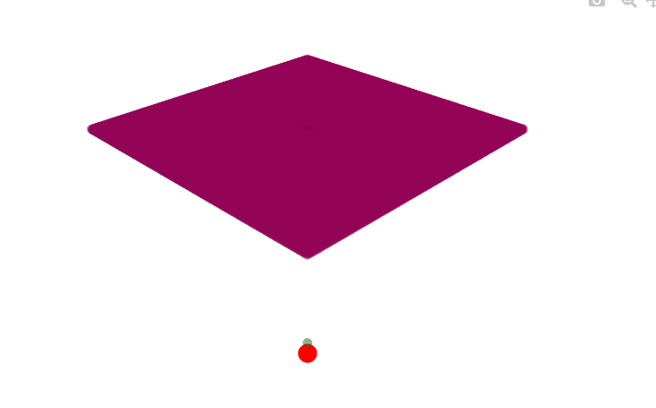
matyas函数
tf = single.matyas


plot_parameters = {


    'min_values': (-10, -10),
    'max_values': (10, 10),
    'step': (0.1, 0.1),
    'solution': [(0, 0)],
    'proj_view': '3D',
    'view': 'notebook'
}
graphs.plot_single_function(target_function = tf, **plot_parameters)
如下:
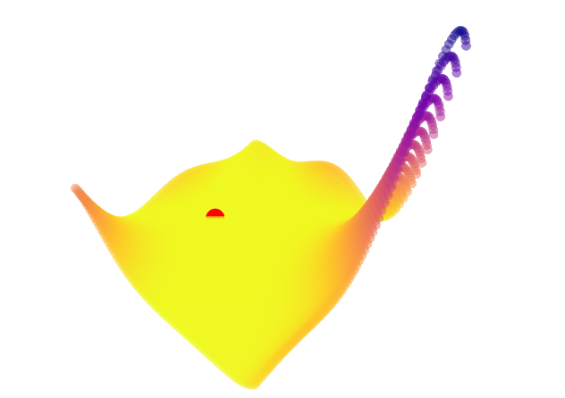
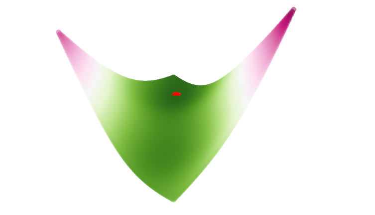
换个颜色:
tf = single.mccormick


plot_parameters = {


    'min_values': (-1.5, -3),
    'max_values': (4, 4),
    'step': (0.05, 0.05),
    'solution': [(-0.54719, -1.54719)],
    'proj_view': '3D',
    'view': 'notebook'
}
graphs.plot_single_function(target_function = tf, **plot_parameters)
如下:
levi_13函数
tf = single.levi_13


plot_parameters = {


    'min_values': (-10, -10),
    'max_values': (10, 10),
    'step': (0.1, 0.1),
    'solution': [(1, 1)],
    'proj_view': '3D',
    'view': 'notebook'
}
graphs.plot_single_function(target_function = tf, **plot_parameters)
绘制如下:
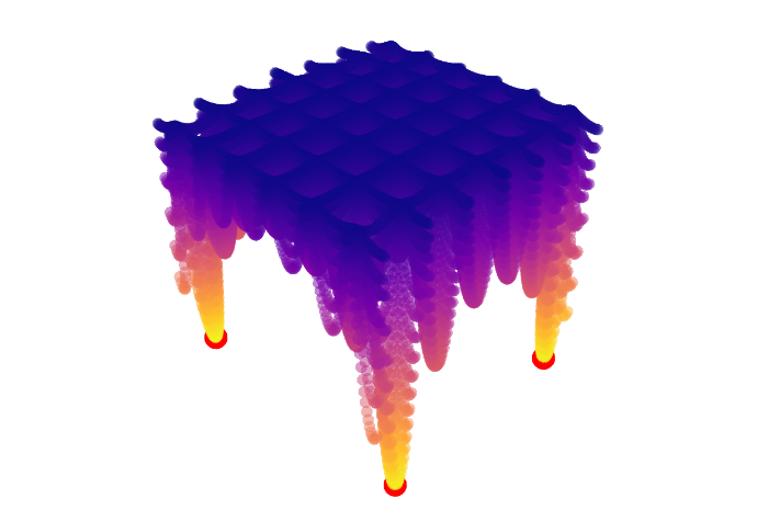
rastrigin函数
tf = single.rastrigin


plot_parameters = {


    'min_values': (-5.12, -5.12),
    'max_values': (5.12, 5.12),
    'step': (0.1, 0.1),
    'solution': [(0, 0)],
    'proj_view': '3D',
    'view': 'notebook'
}
graphs.plot_single_function(target_function = tf, **plot_parameters)
绘制如下:
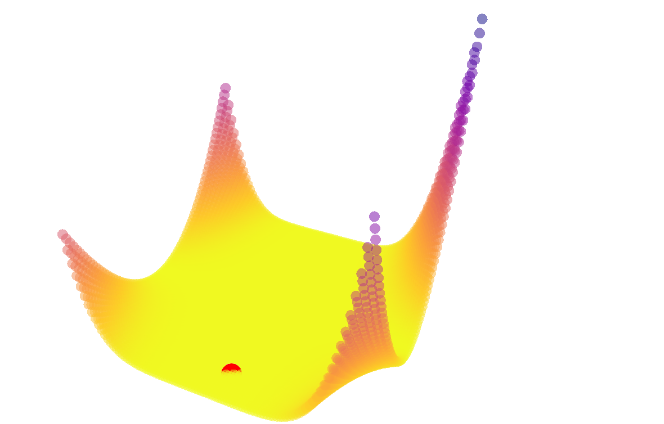
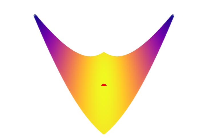
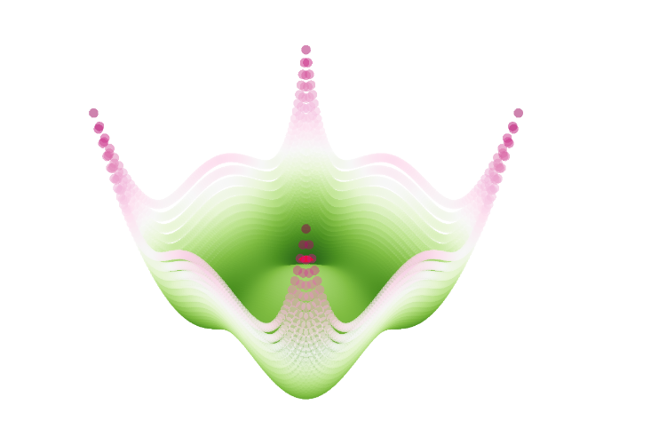
rosenbrocks_valley函数
tf = single.rosenbrocks_valley


plot_parameters = {


    'min_values': (-5, -5),
    'max_values': (5, 5),
    'step': (0.1, 0.1),
    'solution': [(1, 1)],
    'proj_view': '3D',
    'view': 'notebook'
}
graphs.plot_single_function(target_function = tf, **plot_parameters)
绘制如下:
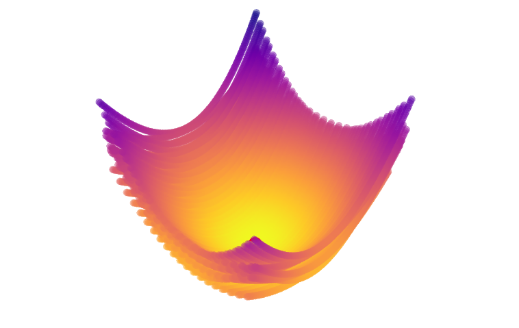
schaffer_2函数
tf = single.schaffer_2


plot_parameters = {


    'min_values': (-100, -100),
    'max_values': (100, 100),
    'step': (1, 1),
    'solution': [(0, 0)],
    'proj_view': '3D',
    'view': 'notebook'
}
graphs.plot_single_function(target_function = tf, **plot_parameters)
绘制如下:
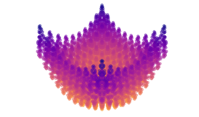
放大一点:
tf = single.schaffer_4


plot_parameters = {


    'min_values': (-100, -100),
    'max_values': (100, 100),
    'step': (1, 1),
    'solution': [(0, 1.25313), (0, -1.25313), (1.25313, 0), (-1.25313, 0)],
    'proj_view': '3D',
    'view': 'notebook'
}
graphs.plot_single_function(target_function = tf, **plot_parameters)
如下:
再做修改:
tf = single.schaffer_6


plot_parameters = {


    'min_values': (-100, -100),
    'max_values': (100, 100),
    'step': (1, 1),
    'solution': [(0, 0)],
    'proj_view': '3D',
    'view': 'notebook'
}
graphs.plot_single_function(target_function = tf, **plot_parameters)
如下:
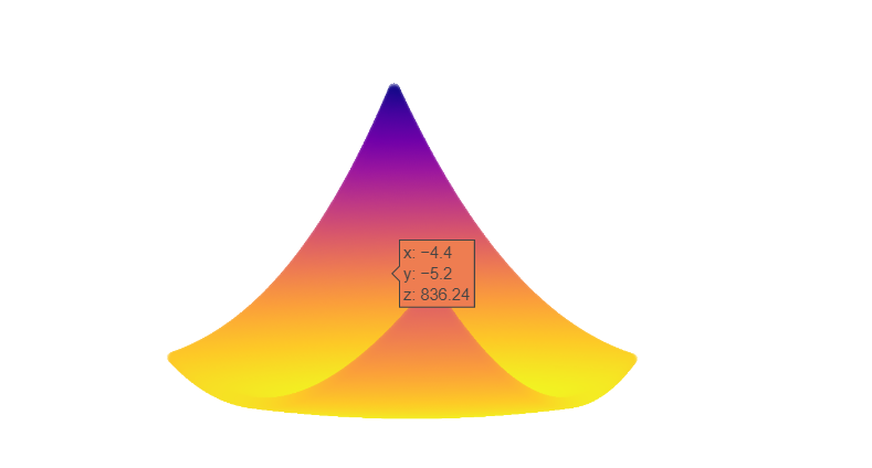
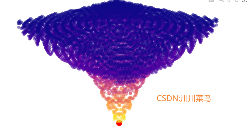
schwefel函数
tf = single.schwefel


plot_parameters = {


    'min_values': (-500, -500),
    'max_values': (500, 500),
    'step': (5, 5),
    'solution': [(420.9687, 420.9687)],
    'proj_view': '3D',
    'view': 'notebook'
}
graphs.plot_single_function(target_function = tf, **plot_parameters)
如下:
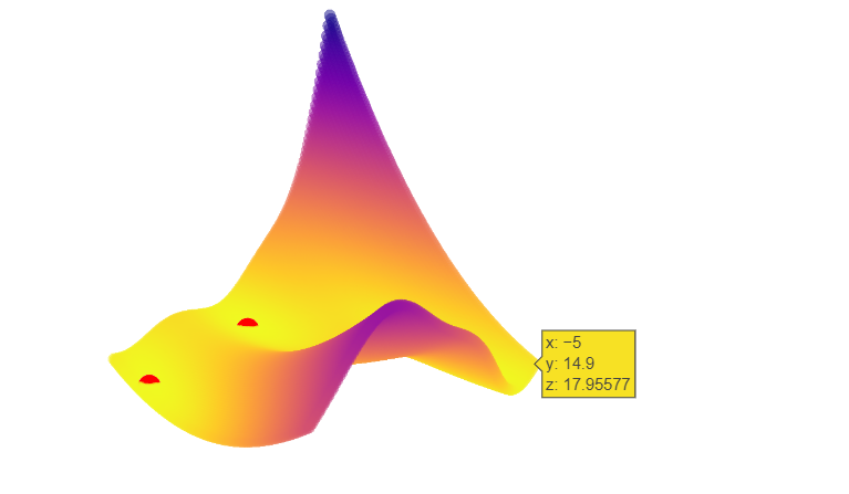
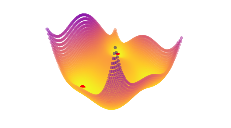
six_hump_camel_back函数
tf = single.six_hump_camel_back


plot_parameters = {


    'min_values': (-3, -2),
    'max_values': (3, 2),
    'step': (0.1, 0.1),
    'solution': [(0.0898, -0.7126), (-0.0898, 0.7126)],
    'proj_view': '3D',
    'view': 'notebook'
}
graphs.plot_single_function(target_function = tf, **plot_parameters)
绘制如下:
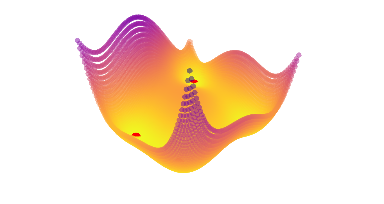
styblinski_tang函数
tf = single.styblinski_tang


plot_parameters = {


    'min_values': (-5, -5),
    'max_values': (5, 5),
    'step': (0.1, 0.1),
    'solution': [(-2.903534, -2.903534)],
    'proj_view': '3D',
    'view': 'notebook'
}
graphs.plot_single_function(target_function = tf, **plot_parameters)
绘制如下:
zakharov函数
tf = single.zakharov


plot_parameters = {


    'min_values': (-5, -5),
    'max_values': (10, 10),
    'step': (0.1, 0.1),
    'solution': [(0, 0)],
    'proj_view': '3D',
    'view': 'notebook'
}
graphs.plot_single_function(target_function = tf, **plot_parameters)
绘制如下:
你喜欢哪个函数呢?
评论区留言说说哪个函数你更喜欢呢?数学是不是距离我们如此近,如此的优美,越发变得简单了?