rWCVP生成可发表级别的物种发现记录矩阵
介绍
世界维管植物名录(WCVP)提供了已知的>340,000种维管植物物种的分布数据。该分布数据可用于构建植物物种名录的发现记录矩阵,rWCVP可以提供帮助。
除了 rWCVP 之外,还可以使用 tidyverse 包进行数据操作和绘图,并使用 gt 包来格式化表格。
先做好准备工作
library(rWCVP)
library(tidyverse)
library(gt)
在此示例中,使用==管道运算符 (%>%) 和 dplyr语法 ==- 如果不熟悉这些,我建议查看 https://dplyr.tidyverse.org/ 和其中的一些帮助页面。
1. 查询一组示例数据
对于这个例子,我们没有想要检查的特定区域或植物组,但这让我们有机会展示rWCVP中的其他功能之一!
我们想要一组物种,a)不太大,b)分布在几个WGSRPD 3级区域。巴西就是不错的选择,因为它有五个3级区域(对于这个目的来说,这是一个不错的数字,因为该表格将适合纵向页面)。让我们看看是否有一些大小不错的示例属,使用 wcvp_summary 函数:
wcvp_summary(taxon = "Myrtaceae", taxon_rank = "family", area=get_wgsrpd3_codes("Brazil"), grouping_var = "genus")%>%wcvp_summary_gt()
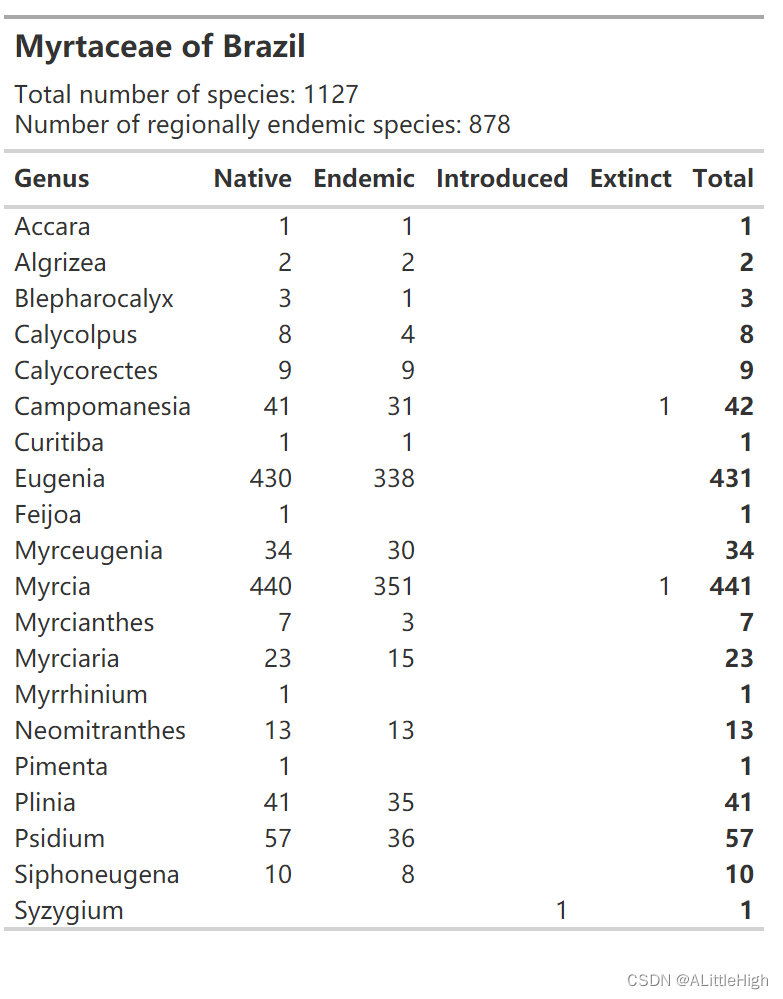
Calycolpus看起来又漂亮又整齐——让我们看看这 8 个物种是如何分布在 5 个区域的。
我们可以使用相同的函数,但限制我们的分类单元并将我们的分组变量更改为 area。
wcvp_summary(taxon = "Calycolpus", taxon_rank = "genus", area=get_wgsrpd3_codes("Brazil"), grouping_var = "area_code_l3")%>%wcvp_summary_gt()
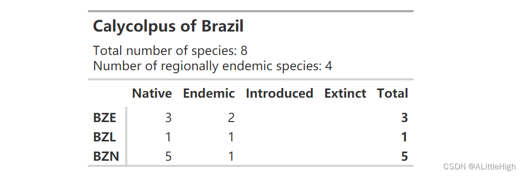
嗯,也许有点太小了 - 它只出现在 5 个区域中的 3 个。Myrciaria呢?
wcvp_summary(taxon = "Myrciaria", taxon_rank = "genus", area=get_wgsrpd3_codes("Brazil"), grouping_var = "area_code_l3")%>%wcvp_summary_gt()
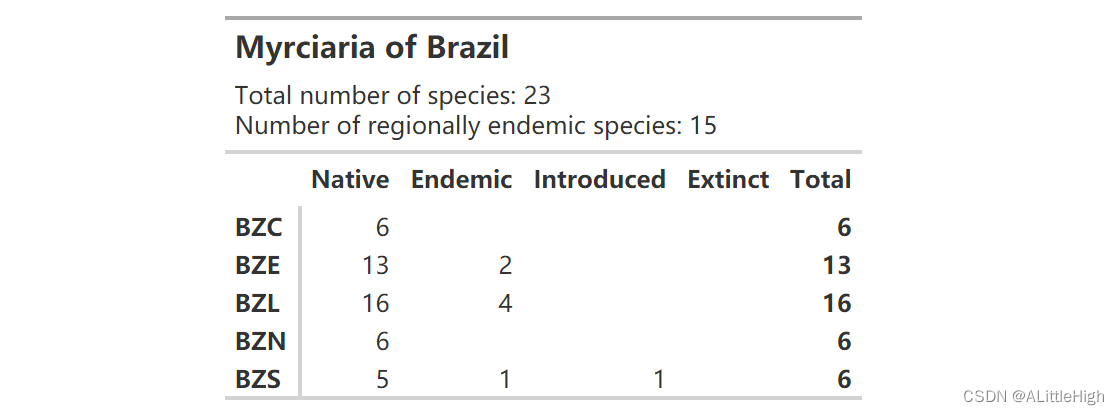
2. 生成和格式化出现矩阵
为该属生成出现矩阵就像使用 generate_occurence_matrix 函数一样简单。
m = wcvp_occ_mat(taxon = "Myrciaria", taxon_rank = "genus", area=get_wgsrpd3_codes("Brazil"))
# A tibble: 23 × 7
   plant_name_id taxon_name             BZC   BZE   BZL   BZN   BZS
           <dbl> <chr>                <dbl> <dbl> <dbl> <dbl> <dbl>
 1        473796 Myrciaria alagoana       0     1     0     0     0
 2        534878 Myrciaria alta           0     0     1     0     0
 3        534776 Myrciaria cambuca        0     1     1     0     0
 4        131799 Myrciaria cordata        0     0     0     1     0
 5        131802 Myrciaria cuspidata      1     1     1     0     1
 6        131803 Myrciaria delicatula     1     0     1     0     1
 7        131806 Myrciaria disticha       0     1     1     0     0
 8        131810 Myrciaria dubia          1     0     0     1     0
 9        491614 Myrciaria evanida        0     0     1     0     0
10        131814 Myrciaria ferruginea     0     1     1     0     0
# ℹ 13 more rows
# ℹ Use `print(n = ...)` to see more rows
没关系,但是我们可以使用 gt 包让它更漂亮。让我们执行以下操作:
- 删除 WCVP ID 列
- 将taxon_id更改为“物种”
- 使物种名称为斜体
- 加粗列标题
- 减少文本周围的空间,使字体大小为 12
- 删除内部边框
- 将 1 和 0 更改为 X 和空白
m_gt = m %>%
  select(-plant_name_id) %>%
  gt() %>%
  cols_label(
    taxon_name = "Species"
  ) %>%
  tab_style(
    style = cell_text(style = "italic"),
    locations = cells_body(columns = taxon_name)
  ) %>%
  tab_options(
    column_labels.font.weight = "bold",
    data_row.padding = px(1),
    table.font.size = 12,
    table_body.hlines.color = "transparent",
  ) %>%
  text_transform(
    locations = cells_body(),
    fn = function(x) {


      ifelse(x==0, "", x)
    }
  ) %>%
  text_transform(
    locations = cells_body(),
    fn = function(x){


      ifelse(x==1, "X", x)
    }
  )

m_gt
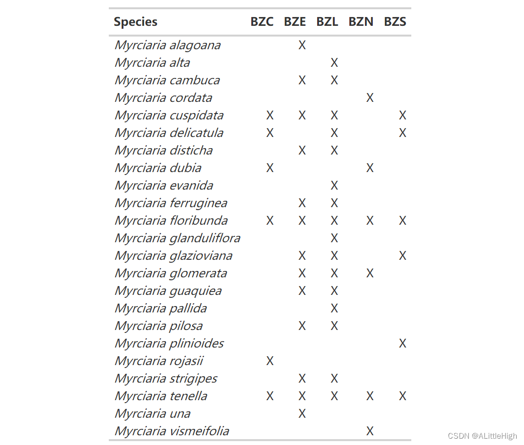
好多了!我们可以将此 gt 表另存为 HTML 表或图片。如果我们打算再制作几个表格,我们可以通过将表格样式保存为主题来节省空间(有关更多详细信息,请参阅 https://themockup.blog/posts/2020-09-26-functions-and-themes-for-gt-tables/)
occ_mat_theme <- function(x){


  x %>% cols_label(
    taxon_name = "Species"
  ) %>%
  #make species names italic
        tab_style(
        style=cell_text(style="italic"),
        locations = cells_body(
          columns= taxon_name
        )
      ) %>%
  tab_options(
    # some nice formatting
        column_labels.font.weight = "bold",
        data_row.padding = px(1),
        table.font.size = 12,
        table_body.hlines.color = "transparent",
        ) %>%
  # change the zeroes into blanks
      text_transform(
        locations = cells_body(),
        fn = function(x){


          ifelse(x == 0, "", x)
        }
      ) %>%
  # change the 1s into X
        text_transform(
        locations = cells_body(),
        fn = function(x){


          ifelse(x == 1, "X", x)
        }
      )
}
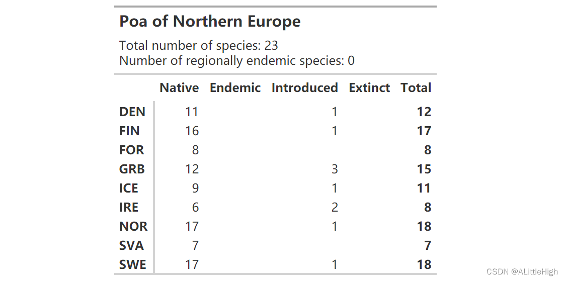
gt() 的最大问题是它不支持 Word - 要直接导出到 docx 文件,请查看 flextable 。包括或排除发生类型 如果我们只想知道本地或引进物种怎么办?此函数可以选择筛选其中一个。巴西Myrciaria在这方面看起来不是很有趣(我们可以从汇总表中看到只引入了一个物种),所以让我们看看一个更具入侵性的群体 - 北欧的Poa(2级区域)。
wcvp_summary(taxon = "Poa", taxon_rank = "genus", area=get_wgsrpd3_codes("Northern Europe"), grouping_var = "area_code_l3") %>% wcvp_summary_gt()
还有一些工作要做。首先,让我们只看本地物种:
p = wcvp_occ_mat(taxon = "Poa", taxon_rank = "genus", area=get_wgsrpd3_codes("Northern Europe"), introduced = FALSE, extinct = FALSE, location_doubtful = FALSE)
p
# A tibble: 20 × 11
   plant_name_id taxon_name        DEN   FIN   FOR   GRB   ICE   IRE
           <dbl> <chr>           <dbl> <dbl> <dbl> <dbl> <dbl> <dbl>
 1        435004 Poa abbreviata      0     0     0     0     0     0
 2        435078 Poa alpigena        0     1     1     0     1     0
 3        435085 Poa alpina          0     1     1     1     1     1
 4        435167 Poa angustifol…     1     1     0     1     0     0
 5        435194 Poa annua           1     1     1     1     1     1
 6        435235 Poa arctica         0     1     0     0     0     0
 7        435458 Poa bulbosa         1     1     0     1     0     0
 8        435622 Poa compressa       1     1     0     0     0     0
 9        435932 Poa flexuosa        0     0     0     1     1     0
10        435996 Poa glauca          0     1     1     1     1     0
11        436089 Poa hartzii         0     0     0     0     0     0
12        436146 Poa humilis         1     1     1     1     1     1
13        436189 Poa infirma         0     0     0     1     0     0
14        436383 Poa lindebergii     0     1     0     0     0     0
15        436600 Poa nemoralis       1     1     1     1     1     1
16        436739 Poa palustris       1     1     0     1     0     0
17        436906 Poa pratensis       1     1     1     1     1     1
18        437092 Poa remota          1     1     0     0     0     0
19        437424 Poa supina          1     1     0     0     0     0
20        437547 Poa trivialis       1     1     1     1     1     1
# ℹ 3 more variables: NOR <dbl>, SVA <dbl>, SWE <dbl>
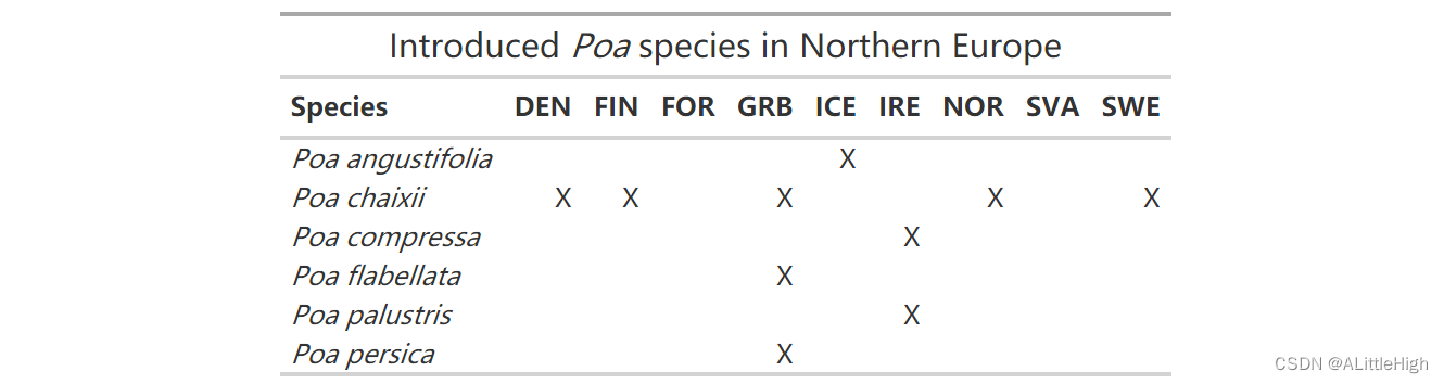
我们可以像上面一样格式化这个矩阵,但让我们跳过那些步骤,直接处理引入的物种。我们正在做与以前相同的格式设置,但也添加一个标题 - html 函数可以将我们的属名和所有内容斜体化!
p = wcvp_occ_mat(taxon = "Poa", taxon_rank = "genus", area=get_wgsrpd3_codes("Northern Europe"),native = FALSE, introduced = TRUE, extinct = FALSE, location_doubtful = FALSE)
p %>%
  select(-plant_name_id) %>% #remove ID col
  gt() %>%
  occ_mat_theme() %>%  #the theme we defined above
  #add a header
  tab_header(title=html("Introduced <em>Poa</em> species in Northern Europe"))
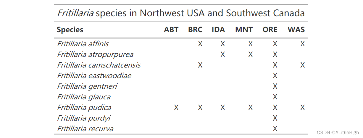
3. 额外地对国家进行处理
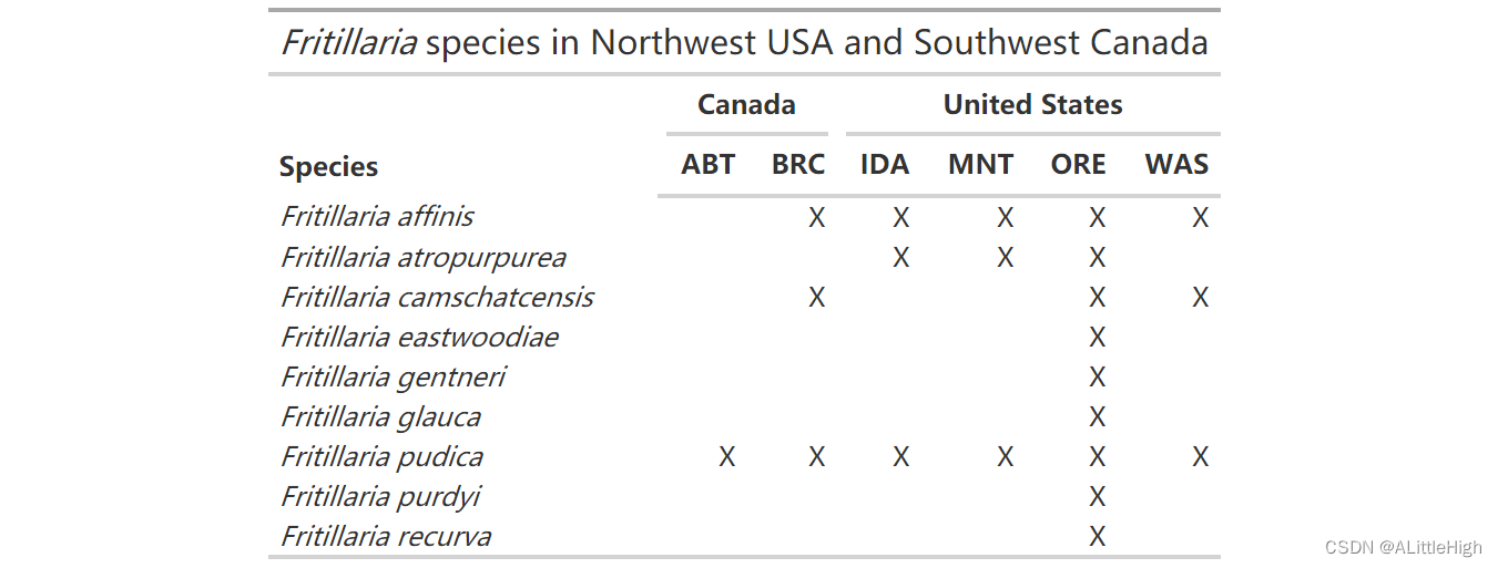
使用 gt 创建的表非常灵活 - 假设我们想查看美加边境出现的记录:
f = wcvp_occ_mat("Fritillaria", "genus", area=c("WAS","ORE","IDA","MNT","ABT","BRC"))
f_gt = f %>%
  select(-plant_name_id) %>%
  gt() %>%
  occ_mat_theme() %>%
  tab_header(title = html("<em>Fritillaria</em> species in Northwest USA and Southwest Canada"))
f_gt
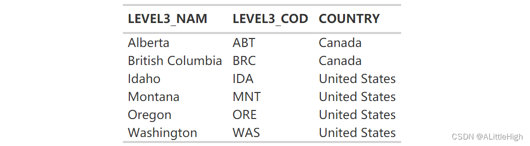
了解哪些代码在美国,哪些在加拿大非常有用。我们可以使用 rWCVP 中包含的数据来创建检索表。
wgsrpd_mapping %>%
  filter(LEVEL3_COD %in% c("WAS","ORE","IDA","MNT","ABT","BRC")) %>%
  select(LEVEL3_NAM, LEVEL3_COD, COUNTRY) %>%
  gt() %>%
  tab_options(
    column_labels.font.weight = "bold",
    data_row.padding = px(1),
    table.font.size = 12,
    table_body.hlines.color = "transparent",
  )
不过,将其放在发生矩阵上确实会更好。输入 tab_spanner():
f_gt %>%
  tab_spanner(label = "United States", columns = c(IDA, MNT, ORE, WAS)) %>%
  tab_spanner(label = "Canada", columns = c(ABT, BRC))
gt 还有很多事情可以做 - 请参阅 https://gt.rstudio.com/ 以获取帮助、示例和文档。