====================== ExpressionSet
 class(gset)
[1] "list"
#取列表中的元素
a=gset[[1]]
class(a)
dat=exprs(a) #a现在是一个对象,取a这个对象通过看说明书知道要用exprs这个函数
pd=pData(a) #用pData来提取临床信息

fd=fData(gset[[1]])
Introduction
The ExpressionSet is generally used for array-based experiments, where the rows are features, and the SummarizedExperiment is generally used for sequencing-based experiments, where the rows are GenomicRanges. ExpressionSet is in the Biobase library.
There’s a library GEOquery which lets you pull down ExpressionSets by identifier.
library(Biobase) #Download data from GEO library(GEOquery) geoq <- getGEO("GSE9514") #The list has a single element #Save it to letter e for simplicity names(geoq)## [1] "GSE9514_series_matrix.txt.gz"e <- geoq[[1]]ExpressionSet
ExpressionSets are basically matrices with a lot of metadata around them. Here, we have a matrix which is 9,000 by 8. It has phenotypic data, feature and annotation information. You can use the functions dim, ncol, nrow to have the dimension, the number of columns and rows respectively.The matrix of the expression data, is stored in the exprs slot and you can access that with the exprs function. The phenotypic data, can be accessed using pData and this gives us a data frame, which is information about the samples, including the accession number, the submission date, etc). The feature data is accessible with fData function and this is information about genes or probe sets. The names of the data in the feature data are, for example, the gene title, the gene symbol, the ENREZ_Gene_ID or Gene Ontology information, which might be useful for downstream analysis.
#The expression matrix exprs(e)[1:3,1:3]## GSM241146 GSM241147 GSM241148 ## 10000_at 15.33 9.459 7.985 ## 10001_at 283.47 300.729 270.016 ## 10002_i_at 2569.45 2382.815 2711.814#Phenotypic data: information about the samples pData(e)[1:3,1:6]## title ## GSM241146 hem1 strain grown in YPD with 250 uM ALA (08-15-06_Philpott_YG_S98_1) ## GSM241147 WT strain grown in YPD under Hypoxia (08-15-06_Philpott_YG_S98_10) ## GSM241148 WT strain grown in YPD under Hypoxia (08-15-06_Philpott_YG_S98_11) ## geo_accession status submission_date ## GSM241146 GSM241146 Public on Nov 06 2007 Nov 02 2007 ## GSM241147 GSM241147 Public on Nov 06 2007 Nov 02 2007 ## GSM241148 GSM241148 Public on Nov 06 2007 Nov 02 2007 ## last_update_date type ## GSM241146 Aug 14 2011 RNA ## GSM241147 Aug 14 2011 RNA ## GSM241148 Aug 14 2011 RNAdim(pData(e))## [1] 8 31#Column names of the phenotypic data names(pData(e))## [1] "title" "geo_accession" ## [3] "status" "submission_date" ## [5] "last_update_date" "type" ## [7] "channel_count" "source_name_ch1" ## [9] "organism_ch1" "characteristics_ch1" ## [11] "molecule_ch1" "extract_protocol_ch1" ## [13] "label_ch1" "label_protocol_ch1" ## [15] "taxid_ch1" "hyb_protocol" ## [17] "scan_protocol" "description" ## [19] "data_processing" "platform_id" ## [21] "contact_name" "contact_email" ## [23] "contact_department" "contact_institute" ## [25] "contact_address" "contact_city" ## [27] "contact_state" "contact_zip/postal_code" ## [29] "contact_country" "supplementary_file" ## [31] "data_row_count"#Feature data : information about genes or probe sets fData(e)[1:3,1:3]## ID ORF SPOT_ID ## 10000_at 10000_at YLR331C ## 10001_at 10001_at YLR332W ## 10002_i_at 10002_i_at YLR333Cdim(fData(e))## [1] 9335 17names(fData(e))## [1] "ID" "ORF" ## [3] "SPOT_ID" "Species Scientific Name" ## [5] "Annotation Date" "Sequence Type" ## [7] "Sequence Source" "Target Description" ## [9] "Representative Public ID" "Gene Title" ## [11] "Gene Symbol" "ENTREZ_GENE_ID" ## [13] "RefSeq Transcript ID" "SGD accession number" ## [15] "Gene Ontology Biological Process" "Gene Ontology Cellular Component" ## [17] "Gene Ontology Molecular Function"head(fData(e)$"Gene Symbol")## [1] JIP3 MID2 RPS25B NUP2 ## 4869 Levels: ACO1 ARV1 ATP14 BOP2 CDA1 CDA2 CDC25 CDC3 CDD1 CTS1 ... Il4head(rownames(e))## [1] "10000_at" "10001_at" "10002_i_at" "10003_f_at" "10004_at" ## [6] "10005_at"
========================================Summarized Experiment
library(SummarizedExperiment)
data(airway, package="airway")
se <- airway
se
assays(se)$counts
assays(se)
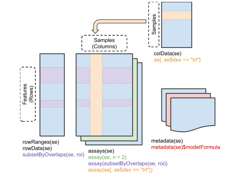
assays(se)是assays(se)对象的中心部分,在测序数据中相当于行是基因或探针,列是样品名,表格中是表达矩阵,assays(se)中实际上可以储存多个表达矩阵,如同时包含蛋白质组、RNAseq、表观遗传等测序数据,通过assays(se)$矩阵名的方式来进行调用,如果只有一种类型的表达矩阵用assays(se)语句就可以了。
‘Row’ (regions-of-interest) data
The rowRanges() accessor is used to view the range information for a RangedSummarizedExperiment. (Note if this were the parent SummarizedExperiment class we’d use rowData()). The data are stored in a GRangesList object, where each list element corresponds to one gene transcript and the ranges in each GRanges correspond to the exons in the transcript.
rowRanges(se)
rowRanges(se)
顾名思义,这是于行相关的一个数据表格,储存的就是基因或者探针对应的基因组区域,如下图。如果SummarizedExperiment具有这一个属性的表格的话,我们也会称之为 RangedSummarizedExperiment对象,也就是对基因位置信息的注释不是一定需要具备的属性,因为在很多研究中,我们并不关注基因在染色体中的哪个区域。
colData(se)
列相关信息,也就是样品相关的信息,因为表达矩阵中可能仅仅具有样品名,这些样品可能具有不同的属性,比如说来自于性别、年龄、BMI等数据不同的个体,或者是细胞的培养条件不同,样品的处理方法不同等,我们都可以colData(se)表格中记录这些差异信息。
metadata(se)
也就是关于实验的备注信息,在哪做实验的,使用了什么仪器等,metadata中的信息是可以自定义修改和添加的,和rowRanges(se)不是se对象必须具备的属性。Summarized Experiment
I’m going to load a bioconductor annotation package, which is the parathyroid SummarizedExperiment library. The loaded data is a SummarizedExperiment, which summarizes counts of RNA sequencing reads in genes for an experiment on human cell culture. The SummarizedExperiment object has 63,000 rows, which are genes, and 27 columns, which are samples, and the matrix, in this case, is called counts. And we have the row names, which are ensemble genes, and metadata about the row data, and metadata about the column data.
library(parathyroidSE) #RNA sequencing reads data(parathyroidGenesSE) se <- parathyroidGenesSE se## class: SummarizedExperiment ## dim: 63193 27 ## exptData(1): MIAME ## assays(1): counts ## rownames(63193): ENSG00000000003 ENSG00000000005 ... LRG_98 LRG_99 ## rowData metadata column names(0): ## colnames: NULL ## colData names(8): run experiment ... study sampleassay function can be used get access to the counts of RNA sequencing reads. colData function , the column data, is equivalent to the pData on the ExpressionSet. Each row in this data frame corresponds to a column in the SummarizedExperiment. We can see that there are indeed 27 rows here, which give information about the columns. Each sample in this case is treated with two treatments or control and we can see the number of replicates for each, using the as.numeric function again.
#Dimension of the SummarizedExperiment dim(se)## [1] 63193 27#Get access to the counts of RNA sequencing reads, using assay function. assay(se)[1:3,1:3]## [,1] [,2] [,3] ## ENSG00000000003 792 1064 444 ## ENSG00000000005 4 1 2 ## ENSG00000000419 294 282 164R中SummarizedExperiment包的使用 - 知乎 (zhihu.com)![]() https://zhuanlan.zhihu.com/p/584568742
https://zhuanlan.zhihu.com/p/584568742
Getters and setters
rowRanges()/ (rowData()),colData(),metadata()-
获取rowData(), colData(), metadata()等矩阵
这个在第一部分已经说了方法,不做赘述。可以稍微提一下的是,使用assays(se)中有多个表达矩阵时,可通过中括号的方法进行指定,如assays(se)[[1]]或assay(se, 1)。
assays(se)$counts
assays(se)
================================singlecellexperiment
补充!
| Function | Description |
|---|---|
| rowData(sce) | gene信息 |
| colData(sce) | cell信息 |
| assay(sce, "counts") | 查看counts矩阵 |
| reducedDim(sce, "PCA") | 查看PCA降维table |
| sce$colname | 查看colData的colname, 等价于colData(sce)$colname |
| sce[<rows>, <columns>] | 查看特定行、列 |
修改SingleCellExperiment对象
举个栗子
我们把counts矩阵进行log2(x+1)转换,命名为logcounts。
assay(tung, "logcounts") <- log2(counts(tung) + 1)
# 查看一下
logcounts(tung)[1:4, 1:4]

补充!
| Code | Description |
|---|---|
| assay(sce, "name") <- matrix | 添加新矩阵 |
| rowData(sce) <- data_frame | 替换rowData |
| colData(sce) <- data_frame | 替换colData |
| colData(sce)$column_name <- values | 在colData中添加/替换一个新的列 |
| rowData(sce)$column_name <- values | 在rowData中添加/替换一个新的行 |
| reducedDim(sce, "name") <- matrix | 添加降维矩阵 |

Figure 4.1: Overview of the structure of the SingleCellExperiment class. Each row of the assays corresponds to a row of the rowData (pink shading), while each column of the assays corresponds to a column of the colData and reducedDims (yellow shading).
4.4.2 On the rows
We store feature-level annotation in the rowData slot, a DataFrame where each row corresponds to a gene and contains annotations like the transcript length or gene symbol. We can manually get and set this with the rowData() function, as shown below:
rowData(sce)$Length <- gene.length
rowData(sce)
4.6 Single-cell-specific fields
4.6.1 Background
So far, we have covered the assays (primary data), colData (cell metadata), rowData/rowRanges (feature metadata), and metadata slots (other) of the SingleCellExperiment class. These slots are actually inherited from the SummarizedExperiment parent class (see here for details), so any method that works on a SummarizedExperiment will also work on a SingleCellExperiment object. But why do we need a separate SingleCellExperiment class? This is motivated by the desire to streamline some single-cell-specific operations, which we will discuss in the rest of this section.
4.6.2 Dimensionality reduction results
The reducedDims slot is specially designed to store reduced dimensionality representations of the primary data obtained by methods such as PCA and t�-SNE (see Basic Chapter 4 for more details). This slot contains a list of numeric matrices of low-reduced representations of the primary data, where the rows represent the columns of the primary data (i.e., cells), and columns represent the dimensions. As this slot holds a list, we can store multiple PCA/t�-SNE/etc. results for the same dataset.
In our example, we can calculate a PCA representation of our data using the runPCA() function from scater. We see that the sce now shows a new reducedDim that can be retrieved with the accessor reducedDim().
sce <- scater::logNormCounts(sce)
sce <- scater::runPCA(sce)
dim(reducedDim(sce, "PCA"))