sklearn实战：Kaggle自行车租赁预测（岭回归，支持向量回归，随机森林回归）

import numpy as np
import pandas as pd
import matplotlib.pyplot as plt
import seaborn as sns

df_train=pd.read_csv('kaggle_bike_competition_train.csv',header = 0)

df_train.head(10)

.dataframe tbody tr th:only-of-type { vertical-align: middle; } .dataframe tbody tr th { vertical-align: top; } .dataframe thead th { text-align: right; }

	datetime	season	holiday	workingday	weather	temp	atemp	humidity	windspeed	casual	registered	count
0	2011-01-01 00:00:00	1	0	0	1	9.84	14.395	81	0.0000	3	13	16
1	2011-01-01 01:00:00	1	0	0	1	9.02	13.635	80	0.0000	8	32	40
2	2011-01-01 02:00:00	1	0	0	1	9.02	13.635	80	0.0000	5	27	32
3	2011-01-01 03:00:00	1	0	0	1	9.84	14.395	75	0.0000	3	10	13
4	2011-01-01 04:00:00	1	0	0	1	9.84	14.395	75	0.0000	0	1	1
5	2011-01-01 05:00:00	1	0	0	2	9.84	12.880	75	6.0032	0	1	1
6	2011-01-01 06:00:00	1	0	0	1	9.02	13.635	80	0.0000	2	0	2
7	2011-01-01 07:00:00	1	0	0	1	8.20	12.880	86	0.0000	1	2	3
8	2011-01-01 08:00:00	1	0	0	1	9.84	14.395	75	0.0000	1	7	8
9	2011-01-01 09:00:00	1	0	0	1	13.12	17.425	76	0.0000	8	6	14

字段的名字和类型

df_train.dtypes

datetime object season int64 holiday int64 workingday int64 weather int64 temp float64 atemp float64 humidity int64 windspeed float64 casual int64 registered int64 count int64 dtype: object

df_train.shape

(10886, 12) 看看有没有缺省的字段，好吧，其实那个字段的数据都不缺！

df_train.count()

datetime 10886 season 10886 holiday 10886 workingday 10886 weather 10886 temp 10886 atemp 10886 humidity 10886 windspeed 10886 casual 10886 registered 10886 count 10886 dtype: int64

type(df_train.datetime)

pandas.core.series.Series

# 把月、日、和 小时单独拎出来，放到3列中
df_train['month']=pd.DatetimeIndex(df_train.datetime).month  #创建新的一列'month'，月份
df_train['dayofweek']=pd.DatetimeIndex(df_train.datetime).dayofweek #星期几
df_train['hour']=pd.DatetimeIndex(df_train.datetime).hour #小时

df_train.head(20)

.dataframe tbody tr th:only-of-type { vertical-align: middle; } .dataframe tbody tr th { vertical-align: top; } .dataframe thead th { text-align: right; }

	datetime	season	holiday	workingday	weather	temp	atemp	humidity	windspeed	casual	registered	count	month	dayofweek	hour
0	2011-01-01 00:00:00	1	0	0	1	9.84	14.395	81	0.0000	3	13	16	1	5	0
1	2011-01-01 01:00:00	1	0	0	1	9.02	13.635	80	0.0000	8	32	40	1	5	1
2	2011-01-01 02:00:00	1	0	0	1	9.02	13.635	80	0.0000	5	27	32	1	5	2
3	2011-01-01 03:00:00	1	0	0	1	9.84	14.395	75	0.0000	3	10	13	1	5	3
4	2011-01-01 04:00:00	1	0	0	1	9.84	14.395	75	0.0000	0	1	1	1	5	4
5	2011-01-01 05:00:00	1	0	0	2	9.84	12.880	75	6.0032	0	1	1	1	5	5
6	2011-01-01 06:00:00	1	0	0	1	9.02	13.635	80	0.0000	2	0	2	1	5	6
7	2011-01-01 07:00:00	1	0	0	1	8.20	12.880	86	0.0000	1	2	3	1	5	7
8	2011-01-01 08:00:00	1	0	0	1	9.84	14.395	75	0.0000	1	7	8	1	5	8
9	2011-01-01 09:00:00	1	0	0	1	13.12	17.425	76	0.0000	8	6	14	1	5	9
10	2011-01-01 10:00:00	1	0	0	1	15.58	19.695	76	16.9979	12	24	36	1	5	10
11	2011-01-01 11:00:00	1	0	0	1	14.76	16.665	81	19.0012	26	30	56	1	5	11
12	2011-01-01 12:00:00	1	0	0	1	17.22	21.210	77	19.0012	29	55	84	1	5	12
13	2011-01-01 13:00:00	1	0	0	2	18.86	22.725	72	19.9995	47	47	94	1	5	13
14	2011-01-01 14:00:00	1	0	0	2	18.86	22.725	72	19.0012	35	71	106	1	5	14
15	2011-01-01 15:00:00	1	0	0	2	18.04	21.970	77	19.9995	40	70	110	1	5	15
16	2011-01-01 16:00:00	1	0	0	2	17.22	21.210	82	19.9995	41	52	93	1	5	16
17	2011-01-01 17:00:00	1	0	0	2	18.04	21.970	82	19.0012	15	52	67	1	5	17
18	2011-01-01 18:00:00	1	0	0	3	17.22	21.210	88	16.9979	9	26	35	1	5	18
19	2011-01-01 19:00:00	1	0	0	3	17.22	21.210	88	16.9979	6	31	37	1	5	19

# 那个，保险起见，咱们还是先存一下吧
df_train_origin = df_train

# 抛掉不要的字段
df_train= df_train.drop(['datetime','casual','registered'],axis=1)

df_train.head(5)

.dataframe tbody tr th:only-of-type { vertical-align: middle; } .dataframe tbody tr th { vertical-align: top; } .dataframe thead th { text-align: right; }

	season	holiday	workingday	weather	temp	atemp	humidity	windspeed	count	month	dayofweek	hour
0	1	0	0	1	9.84	14.395	81	0.0	16	1	5	0
1	1	0	0	1	9.02	13.635	80	0.0	40	1	5	1
2	1	0	0	1	9.02	13.635	80	0.0	32	1	5	2
3	1	0	0	1	9.84	14.395	75	0.0	13	1	5	3
4	1	0	0	1	9.84	14.395	75	0.0	1	1	5	4

df_train.shape

(10886, 12)

df_train['count'].head(10)

0    16
1    40
2    32
3    13
4     1
5     1
6     2
7     3
8     8
9    14
Name: count, dtype: int64

type(df_train['count'].values)

numpy.ndarray

回忆鸢尾花案例，sklearn喜欢喂给他的数组是ndarray数组

#数据集一定要注意，不要直接看所有，容易内存爆掉
df_train['count'].values[:10]

array([16, 40, 32, 13,  1,  1,  2,  3,  8, 14], dtype=int64)

df_train_target = df_train['count'].values
df_train_data=df_train.drop(['count'],axis=1).values
print('df_train_data shape is ', df_train_data.shape)
print('df_train_target shape is ', df_train_target.shape)

df_train_data shape is  (10886, 11)
df_train_target shape is  (10886,)

机器学习算法

#这里没有做幅度缩放，因为树模型对数据幅度不敏感
from sklearn import linear_model
#from sklearn import model_selection   #看最新文档都是这个
from sklearn.model_selection import ShuffleSplit
#from sklearn import cross_validation   不用这个
from sklearn.grid_search import GridSearchCV #网格搜索， 能帮助找最好的超参数
from sklearn import svm
from sklearn.ensemble import RandomForestRegressor
from sklearn.learning_curve import learning_curve#回执学习曲线，了解学习状态，方便下一步优化
from sklearn.metrics import explained_variance_score

len(df_train_data)

10886

# 总得切分一下数据咯（训练集和验证集）#ShuffleSplit()交叉验证
cv=model_selection.ShuffleSplit(n_splits=3, test_size=0.2,random_state=0)#n_splits : K折验证的K值

# 各种模型来一圈
print("岭回归")
for train, test in cv.split(df_train_data): 
    svc=linear_model.Ridge().fit(df_train_data[train],df_train_target[train])

    print("train score: {0:.3f}, test score: {1:.3f}\n".format(
        svc.score(df_train_data[train], df_train_target[train]), svc.score(df_train_data[test], df_train_target[test])))
    #{0:.3f} 0表示第一个参数，保留三位小数，是训练集上的得分
    #{1:.3f} 1表示测试集上的得分

print("支持向量回归/SVR(kernel='rbf',C=10,gamma=.001)")
for train, test in cv.split(df_train_data):

    svc = svm.SVR(kernel ='rbf', C = 10, gamma = .001).fit(df_train_data[train], df_train_target[train])
    print("train score: {0:.3f}, test score: {1:.3f}\n".format(
        svc.score(df_train_data[train], df_train_target[train]), svc.score(df_train_data[test], df_train_target[test])))

print("随机森林回归/Random Forest(n_estimators = 100)")    
for train, test in cv.split(df_train_data):    
    svc = RandomForestRegressor(n_estimators = 100).fit(df_train_data[train], df_train_target[train])
    print("train score: {0:.3f}, test score: {1:.3f}\n".format(
        svc.score(df_train_data[train], df_train_target[train]), svc.score(df_train_data[test], df_train_target[test])))

岭回归
train score: 0.339, test score: 0.332

train score: 0.330, test score: 0.370

train score: 0.342, test score: 0.320

支持向量回归/SVR(kernel='rbf',C=10,gamma=.001)
train score: 0.417, test score: 0.408

train score: 0.406, test score: 0.452

train score: 0.419, test score: 0.390

随机森林回归/Random Forest(n_estimators = 100)
train score: 0.982, test score: 0.865

train score: 0.981, test score: 0.881

train score: 0.982, test score: 0.867

用GridSearch找参数(用网格搜索选择最优超参数)

X = df_train_data
y = df_train_target
X_train, X_test, y_train, y_test = model_selection.train_test_split(
    X, y, test_size=0.2, random_state=0)    #找超参数，不用交叉验证了，直接切分数据就行
parameters = {'n_estimators':[10,100,500]}
svc=RandomForestRegressor()
clf=GridSearchCV(svc, parameters, cv=5, scoring='r2')   #cv几折交叉验证
clf.fit(X_train,y_train)

GridSearchCV(cv=5, error_score='raise',
       estimator=RandomForestRegressor(bootstrap=True, criterion='mse', max_depth=None,
           max_features='auto', max_leaf_nodes=None,
           min_impurity_decrease=0.0, min_impurity_split=None,
           min_samples_leaf=1, min_samples_split=2,
           min_weight_fraction_leaf=0.0, n_estimators=10, n_jobs=1,
           oob_score=False, random_state=None, verbose=0, warm_start=False),
       fit_params={}, iid=True, n_jobs=1,
       param_grid={'n_estimators': [10, 100, 500]},
       pre_dispatch='2*n_jobs', refit=True, scoring='r2', verbose=0)

 print(clf.best_estimator_)  

RandomForestRegressor(bootstrap=True, criterion='mse', max_depth=None,
           max_features='auto', max_leaf_nodes=None,
           min_impurity_decrease=0.0, min_impurity_split=None,
           min_samples_leaf=1, min_samples_split=2,
           min_weight_fraction_leaf=0.0, n_estimators=500, n_jobs=1,
           oob_score=False, random_state=None, verbose=0, warm_start=False)

学习曲线

%matplotlib inline

def plot_learning_curve(estimator, title, X, y, ylim=None, cv=None,
                        n_jobs=1, train_sizes=np.linspace(.1, 1.0, 5)):

    plt.figure()
    plt.title(title)
    if ylim is not None:
        plt.ylim(*ylim)
    plt.xlabel("Training examples")
    plt.ylabel("Score")
    train_sizes, train_scores, test_scores = learning_curve(
        estimator, X, y, cv=cv, n_jobs=n_jobs, train_sizes=train_sizes)
    train_scores_mean = np.mean(train_scores, axis=1)
    train_scores_std = np.std(train_scores, axis=1)
    test_scores_mean = np.mean(test_scores, axis=1)
    test_scores_std = np.std(test_scores, axis=1)
    plt.grid()

    plt.fill_between(train_sizes, train_scores_mean - train_scores_std,
                     train_scores_mean + train_scores_std, alpha=0.1,
                     color="r")
    plt.fill_between(train_sizes, test_scores_mean - test_scores_std,
                     test_scores_mean + test_scores_std, alpha=0.1, color="g")
    plt.plot(train_sizes, train_scores_mean, 'o-', color="r",
             label="Training score")
    plt.plot(train_sizes, test_scores_mean, 'o-', color="g",
             label="Cross-validation score")

    plt.legend(loc="best")
    return plt

title = "Learning Curves (Random Forest, n_estimators = 100)"
# SVC is more expensive so we do a lower number of CV iterations:
cv = ShuffleSplit(n_splits=10, test_size=0.2, random_state=0)
estimator = RandomForestRegressor(n_estimators = 500)
plot_learning_curve(estimator, title, X, y, (0.0, 1.01), cv=cv, n_jobs=4)

plt.show()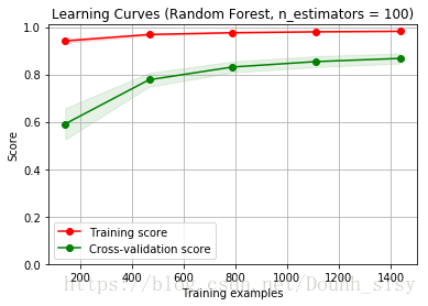

• 随着训练样本的增加，验证分数可以增加
• 训练集和验证测试集直接间隔那么大，这一定是过拟合了

print("随机森林回归/Random Forest(n_estimators=200, max_features=0.6, max_depth=15)")
for train, test in cv.split(X,y): 
    svc = RandomForestRegressor(n_estimators = 200, max_features=0.6, max_depth=15).fit(df_train_data[train], df_train_target[train])
    print("train score: {0:.3f}, test score: {1:.3f}\n".format(
        svc.score(df_train_data[train], df_train_target[train]), svc.score(df_train_data[test], df_train_target[test])))

随机森林回归/Random Forest(n_estimators=200, max_features=0.6, max_depth=15)
train score: 0.984, test score: 0.884

train score: 0.984, test score: 0.893

train score: 0.985, test score: 0.884

train score: 0.985, test score: 0.875

train score: 0.985, test score: 0.897

train score: 0.983, test score: 0.884

train score: 0.985, test score: 0.895

train score: 0.983, test score: 0.887

train score: 0.984, test score: 0.884

train score: 0.982, test score: 0.884