个人学习笔记方便查询
来源:Getting started tutorials
10个知识点:
- pandas库处理什么类型的数据
- 怎么读取和存储数据
- 如何选择DataFrame子集
- 如何在pandas里绘图
- 如何从已有的列创建新列
- 如何计算统计值
- 如何重新设计表格的布局
- 如何从多个表格连接数据
- 如何处理时间序列数据
- 如何处理文本数据
文章目录
(一)pandas库处理什么类型的数据
import pandas as pd
1.pandas数据表

DataFrame:一个二维的数据结构,能存储不同类型的数据(整数,浮点数,类别)
例如存储Titanic的乘客数据,包含名字(字符串),年龄(整数),性别。使用DataFrame创建数据表有三列,列名分别为Name ,Age ,Sex。创建时使用字典。
>>> import pandas as pd
>>> df = pd.DataFrame(
	    {

     "Name": [ "Braund, Mr. Owen Harris","Allen, Mr. William Henry","Bonnell, Miss. Elizabeth"],
          "Age": [22, 35, 58],
          "Sex": ["male", "male", "female"]})
>>> df
                       Name  Age     Sex
0   Braund, Mr. Owen Harris   22    male
1  Allen, Mr. William Henry   35    male
2  Bonnell, Miss. Elizabeth   58  female
2.DataFrame每列都是Series
查看Age列的数据,返回一个Series
>>> df['Age']
0    22
1    35
2    58
Name: Age, dtype: int64
创建Series
>>> ages = pd.Series([22,35,58], name='Age')
>>> ages
0    22
1    35
2    58
Name: Age, dtype: int64
Series没有列标签,只是DataFrame中的某列,但是有行标签
3.DataFrame或者Series操作
想要知道乘客年龄最大值,执行max()操作
>>> df['Age'].max()
58
>>> ages.max()
58
想要知道数据的统计值,Name 和Sex是文本数据,无统计值
>>> df.describe()
             Age
count   3.000000
mean   38.333333
std    18.230012
min    22.000000
25%    28.500000
50%    35.000000
75%    46.500000
max    58.000000
(二)怎么读取和存储数据
1.读数据read

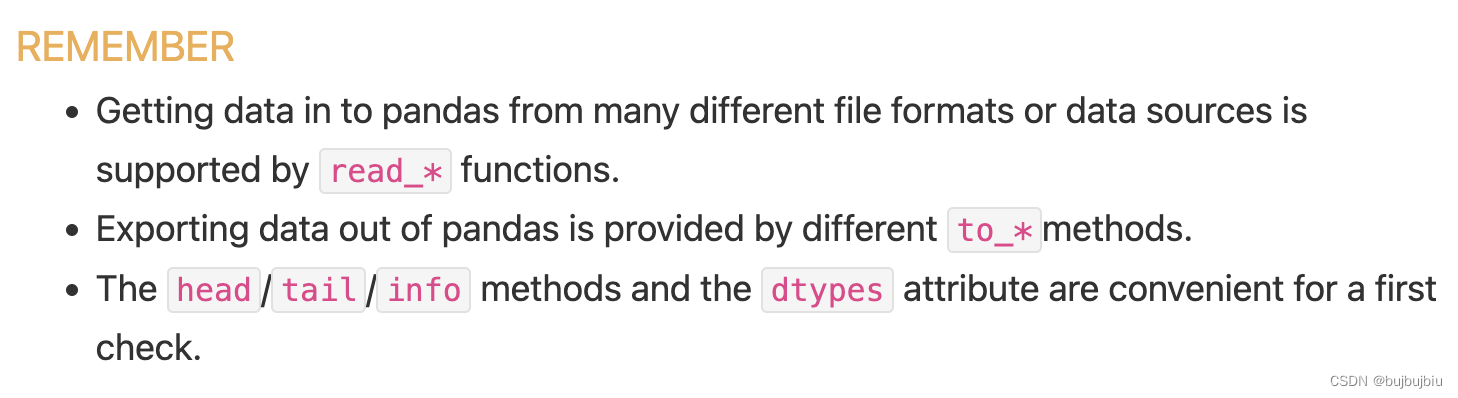
读取Titanic乘客数据,存储在一个CSV文件中。其它格式的文件(csv,excel,sql,json,parquet)都可以读取,格式read_*。默认显示前后5行
>>> titanic = pd.read_csv('/Users/bujibujibiu/Desktop/train.csv')
>>> titanic
     PassengerId  Survived  Pclass  ...     Fare Cabin  Embarked
0              1         0       3  ...   7.2500   NaN         S
1              2         1       1  ...  71.2833   C85         C
2              3         1       3  ...   7.9250   NaN         S
3              4         1       1  ...  53.1000  C123         S
4              5         0       3  ...   8.0500   NaN         S
..           ...       ...     ...  ...      ...   ...       ...
886          887         0       2  ...  13.0000   NaN         S
887          888         1       1  ...  30.0000   B42         S
888          889         0       3  ...  23.4500   NaN         S
889          890         1       1  ...  30.0000  C148         C
890          891         0       3  ...   7.7500   NaN         Q

[891 rows x 12 columns]
指定显示的行,head()和tail()
>>> titanic.head(8)
   PassengerId  Survived  Pclass  ...     Fare Cabin  Embarked
0            1         0       3  ...   7.2500   NaN         S
1            2         1       1  ...  71.2833   C85         C
2            3         1       3  ...   7.9250   NaN         S
3            4         1       1  ...  53.1000  C123         S
4            5         0       3  ...   8.0500   NaN         S
5            6         0       3  ...   8.4583   NaN         Q
6            7         0       1  ...  51.8625   E46         S
7            8         0       3  ...  21.0750   NaN         S

[8 rows x 12 columns]
>>> titanic.tail(8)
     PassengerId  Survived  Pclass  ...    Fare Cabin  Embarked
883          884         0       2  ...  10.500   NaN         S
884          885         0       3  ...   7.050   NaN         S
885          886         0       3  ...  29.125   NaN         Q
886          887         0       2  ...  13.000   NaN         S
887          888         1       1  ...  30.000   B42         S
888          889         0       3  ...  23.450   NaN         S
889          890         1       1  ...  30.000  C148         C
890          891         0       3  ...   7.750   NaN         Q

[8 rows x 12 columns]
查看数据类型
>>> titanic.dtypes
PassengerId      int64
Survived         int64
Pclass           int64
Name            object
Sex             object
Age            float64
SibSp            int64
Parch            int64
Ticket          object
Fare           float64
Cabin           object
Embarked        object
dtype: object
2.存数据to
>>> titanic.to_excel('/Users/bujibujibiu/Desktop/titanic.xlsx', sheet_name='passengers', index=False)
read_*是读数据到pandas,to_*是存储数据到文件里,sheet_name修改表单的名字,默认是Sheet1,index=False不存储行标签,打开titanic.xlsx

再读取titanic.xlsx
>>> titanic = pd.read_excel('/Users/bujibujibiu/Desktop/titanic.xlsx', sheet_name='passengers')
>>> titanic.head()
   PassengerId  Survived  Pclass  ...     Fare Cabin  Embarked
0            1         0       3  ...   7.2500   NaN         S
1            2         1       1  ...  71.2833   C85         C
2            3         1       3  ...   7.9250   NaN         S
3            4         1       1  ...  53.1000  C123         S
4            5         0       3  ...   8.0500   NaN         S

[5 rows x 12 columns]
获取DataFrame的整体信息
>>> titanic.info()
<class 'pandas.core.frame.DataFrame'>
RangeIndex: 891 entries, 0 to 890
Data columns (total 12 columns):
 #   Column       Non-Null Count  Dtype
---  ------       --------------  -----
 0   PassengerId  891 non-null    int64
 1   Survived     891 non-null    int64
 2   Pclass       891 non-null    int64
 3   Name         891 non-null    object
 4   Sex          891 non-null    object
 5   Age          714 non-null    float64
 6   SibSp        891 non-null    int64
 7   Parch        891 non-null    int64
 8   Ticket       891 non-null    object
 9   Fare         891 non-null    float64
 10  Cabin        204 non-null    object
 11  Embarked     889 non-null    object
dtypes: float64(2), int64(5), object(5)
memory usage: 83.7+ KB
(三)如何选择DataFrame子集
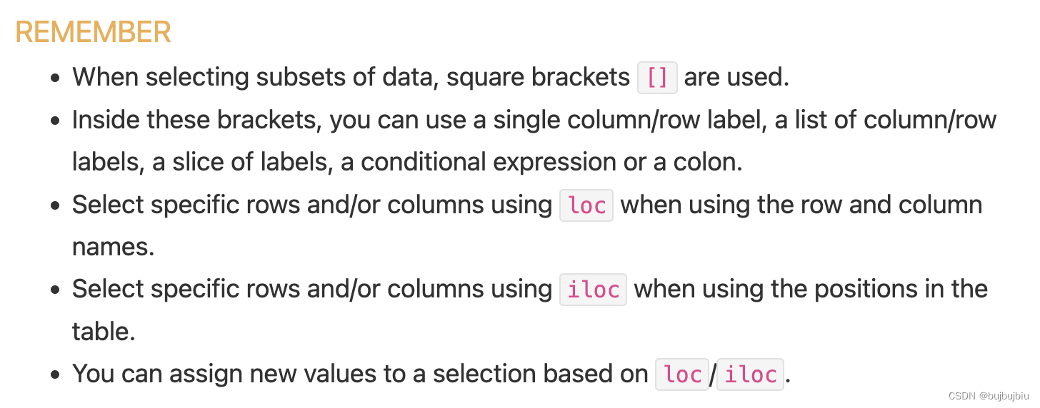
1.选择特定的列

选择乘客的年龄列
>>> ages = titanic['Age']
>>> ages.head()
0    22.0
1    38.0
2    26.0
3    35.0
4    35.0
Name: Age, dtype: float64
列的类型
>>> type(ages)
<class 'pandas.core.series.Series'>
列的形状
>>> ages.shape
(891,)
同时选择多列:年龄和性别
>>> age_sex = titanic[['Age','Sex']]
>>> age_sex.head()
    Age     Sex
0  22.0    male
1  38.0  female
2  26.0  female
3  35.0  female
4  35.0    male
>>> age_sex.shape
(891, 2)
2.过滤指定的行

选择年龄>35的乘客
>>> above_35 = titanic[titanic['Age']>35]
>>> above_35.head()
    PassengerId  Survived  Pclass  ...     Fare Cabin  Embarked
1             2         1       1  ...  71.2833   C85         C
6             7         0       1  ...  51.8625   E46         S
11           12         1       1  ...  26.5500  C103         S
13           14         0       3  ...  31.2750   NaN         S
15           16         1       2  ...  16.0000   NaN         S

[5 rows x 12 columns]
titanic['Age'] > 35判断年龄是否大于35,其它判断符号==,!=,<=,<,返回布尔值,放在[ ]中会返回True的行
>>> titanic['Age'] > 35
0      False
1       True
2      False
3      False
4      False
       ...
886    False
887    False
888    False
889    False
890    False
Name: Age, Length: 891, dtype: bool
选择在船仓2和3的乘客,isin用于判断每行的值是否在列表[2,3]中,与或操作|类似
>>> class_23 = titanic[titanic['Pclass'].isin([2,3])]
>>> class_23.head()
   PassengerId  Survived  Pclass  ...     Fare Cabin  Embarked
0            1         0       3  ...   7.2500   NaN         S
2            3         1       3  ...   7.9250   NaN         S
4            5         0       3  ...   8.0500   NaN         S
5            6         0       3  ...   8.4583   NaN         Q
7            8         0       3  ...  21.0750   NaN         S

[5 rows x 12 columns]
>>> class_23 = titanic[(titanic['Pclass'] == 2) | (titanic['Pclass'] == 3)]
选择年龄不是空值的数据,notna判断是否为空值
>>> age_no_na = titanic[titanic['Age'].notna()]
>>> age_no_na.head()
   PassengerId  Survived  Pclass  ...     Fare Cabin  Embarked
0            1         0       3  ...   7.2500   NaN         S
1            2         1       1  ...  71.2833   C85         C
2            3         1       3  ...   7.9250   NaN         S
3            4         1       1  ...  53.1000  C123         S
4            5         0       3  ...   8.0500   NaN         S

[5 rows x 12 columns]
3.选择指定的行和列
获取年龄大于35岁的乘客的名字,使用loc/iloc操作,前面是想要保留的行,后面的想要选择的列,如果使用列名,行标签,或者条件表达式用loc,如果是数字索引用iloc
>>> adult_names = titanic.loc[titanic['Age'] >35,'Name']
>>> adult_names.head()
1     Cumings, Mrs. John Bradley (Florence Briggs Th...
6                               McCarthy, Mr. Timothy J
11                             Bonnell, Miss. Elizabeth
13                          Andersson, Mr. Anders Johan
15                     Hewlett, Mrs. (Mary D Kingcome)
Name: Name, dtype: object
>>> titanic.iloc[5:9, 2:5]
   Pclass                                               Name     Sex
5       3                                   Moran, Mr. James    male
6       1                            McCarthy, Mr. Timothy J    male
7       3                     Palsson, Master. Gosta Leonard    male
8       3  Johnson, Mrs. Oscar W (Elisabeth Vilhelmina Berg)  female
通过loc/iloc赋新值
>>> titanic.iloc[0:3,3] = 'anonymous'
>>> titanic.head()
   PassengerId  Survived  Pclass  ...     Fare Cabin  Embarked
0            1         0       3  ...   7.2500   NaN         S
1            2         1       1  ...  71.2833   C85         C
2            3         1       3  ...   7.9250   NaN         S
3            4         1       1  ...  53.1000  C123         S
4            5         0       3  ...   8.0500   NaN         S

[5 rows x 12 columns]
(四)如何在pandas里绘图

需要先下载air_quality_no2.csv文件,在OpenAQ上开源,也可以直接去pandas github下载,github只能下载完整的文件,可以将链接https://github.com/pandas-dev/pandas/blob/main/doc/data/air_quality_no2.csv输入到DownGit单独下载

>>> air_quality = pd.read_csv('/Users/bujibujibiu/Desktop/air_quality_no2.csv', index_col=0, parse_dates=True)
>>> air_quality.head()
                     station_antwerp  station_paris  station_london
datetime
2019-05-07 02:00:00              NaN            NaN            23.0
2019-05-07 03:00:00             50.5           25.0            19.0
2019-05-07 04:00:00             45.0           27.7            19.0
2019-05-07 05:00:00              NaN           50.4            16.0
2019-05-07 06:00:00              NaN           61.9             NaN
index_col=0将第一列作为DataFrame的索引,parse_dates=True将列中的日期转换成 Timestamp类型
1.折线图
pandas会默认创建数据没列的折线图
>>> air_quality.plot()
<AxesSubplot:xlabel='datetime'>
>>> plt.show()

也可以只显示某列的图
>>> air_quality['station_paris'].plot()
<AxesSubplot:xlabel='datetime'>
>>> plt.show()

2.散点图
可视化London和Pairs的二氧化氮测量值对比图,alpha为不透明度,值为0时为透明状态,默认为1
>>> air_quality.plot.scatter(x='station_london', y='station_paris', alpha=0.5)
<AxesSubplot:xlabel='station_london', ylabel='station_paris'>
>>> plt.show()

除了scatter,还有许多其他图,用dir()显示,dir() 函数不带参数时,返回当前范围内的变量、方法和定义的类型列表;带参数时,返回参数的属性、方法列表。
>>> [method_name for method_name in dir(air_quality.plot) if not method_name.startswith("_")]
['area', 'bar', 'barh', 'box', 'density', 'hexbin', 'hist', 'kde', 'line', 'pie', 'scatter']
调用.plot.*()在Series和DataFrames都能用
3.箱线图
使用DataFrame.plot.box()绘制箱线图
>>> air_quality.plot.box()
<AxesSubplot:>
>>> plt.show()

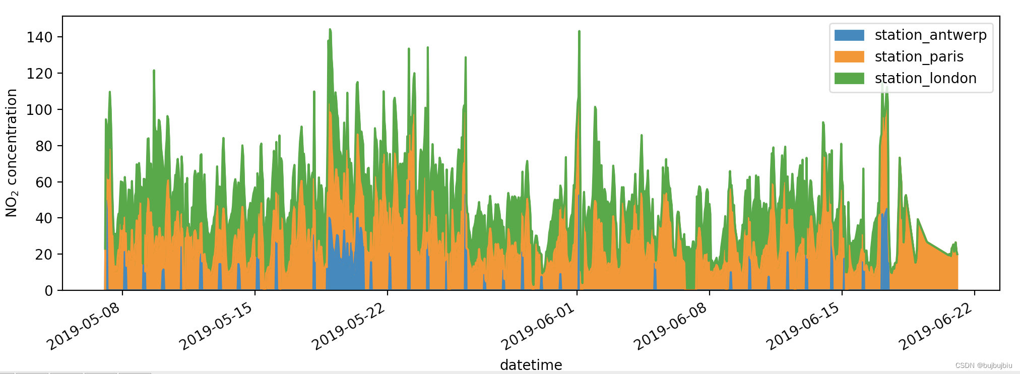
4.多图
想要数据每列在分开的子图里,使用subplots=True
>>> axs = air_quality.plot.area(figsize=(12, 4), subplots=True)
>>> plt.show()

如果想要自己设置图片,可以联合Matplotlib和pandas,每个由pandas创建的图都是Matplotlib对象
# 创建一个空的Matplotlib图像和坐标轴(Matplotlib Figure and Axes)
>>> fig, axs = plt.subplots(figsize=(12,4))
# 使用pandas将数据绘制在定义的图像或者坐标轴上
>>> air_quality.plot.area(ax=axs)
<AxesSubplot:xlabel='datetime'>
# 使用Matplotlib方法设置图片
>>> axs.set_ylabel('NO$_2$ concentration')
Text(0, 0.5, 'NO$_2$ concentration')
>>> fig.savefig('no2_concentrations.png')
>>> plt.show()
(五)如何从已有的列创建新列

1.创建新列
使用前面的空气质量数据,用mg/m3表示London得二氧化氮浓度,转化因子为1.882,创建新列直接使用[]加列名
>>> air_quality['london_mg_per_cubic'] = air_quality['station_london'] * 1.882
>>> air_quality.head()
                     station_antwerp  ...  london_mg_per_cubic
datetime                              ...
2019-05-07 02:00:00              NaN  ...               43.286
2019-05-07 03:00:00             50.5  ...               35.758
2019-05-07 04:00:00             45.0  ...               35.758
2019-05-07 05:00:00              NaN  ...               30.112
2019-05-07 06:00:00              NaN  ...                  NaN

[5 rows x 4 columns]
2.列运算
想要对比Paris和Antwerp并保存到新列
>>> air_quality["ratio_paris_antwerp"] = air_quality['station_paris']  / air_quality["station_antwerp"]
>>> air_quality.head()
                     station_antwerp  ...  ratio_paris_antwerp
datetime                              ...
2019-05-07 02:00:00              NaN  ...                  NaN
2019-05-07 03:00:00             50.5  ...             0.495050
2019-05-07 04:00:00             45.0  ...             0.615556
2019-05-07 05:00:00              NaN  ...                  NaN
2019-05-07 06:00:00              NaN  ...                  NaN

[5 rows x 5 columns]
列之间可以直接运算,其它数学操作符如+, -, *, /和逻辑操作符<, >, ==都能使用,如果想要更复杂的操作,使用apply()函数
3.修改列名
重新命名列使用rename(),rename()对行和列都适用,输入字典提供当前名字和修改的名字
>>> air_quality_renamed = air_quality.rename(columns={

    "station_antwerp": "BETR801","station_paris": "FR04014","station_london": "London Westminster"})
>>> air_quality_renamed.head()
                     BETR801  FR04014  ...  london_mg_per_cubic  ratio_paris_antwerp
datetime                               ...
2019-05-07 02:00:00      NaN      NaN  ...               43.286                  NaN
2019-05-07 03:00:00     50.5     25.0  ...               35.758             0.495050
2019-05-07 04:00:00     45.0     27.7  ...               35.758             0.615556
2019-05-07 05:00:00      NaN     50.4  ...               30.112                  NaN
2019-05-07 06:00:00      NaN     61.9  ...                  NaN                  NaN

[5 rows x 5 columns]
rename()也能实现函数的映射,如使用当前列名的小写
>>> air_quality_renamed = air_quality_renamed.rename(columns=str.lower)
>>> air_quality_renamed.head()
                     betr801  fr04014  ...  london_mg_per_cubic  ratio_paris_antwerp
datetime                               ...
2019-05-07 02:00:00      NaN      NaN  ...               43.286                  NaN
2019-05-07 03:00:00     50.5     25.0  ...               35.758             0.495050
2019-05-07 04:00:00     45.0     27.7  ...               35.758             0.615556
2019-05-07 05:00:00      NaN     50.4  ...               30.112                  NaN
2019-05-07 06:00:00      NaN     61.9  ...                  NaN                  NaN

[5 rows x 5 columns]
(六)如何计算统计值
1.汇总统计

使用titanic数据集,想要知道乘客的平均年龄
>>> titanic = pd.read_csv('/Users/bujibujibiu/Desktop/train.csv')
>>> titanic['Age'].mean()
29.69911764705882
也可以同时选中多列
>>> titanic[['Age','Fare']].median()
Age     28.0000
Fare    14.4542
dtype: float64
查看对应列的统计数据汇总使用describe
>>> titanic[['Age','Fare']].describe()
              Age        Fare
count  714.000000  891.000000
mean    29.699118   32.204208
std     14.526497   49.693429
min      0.420000    0.000000
25%     20.125000    7.910400
50%     28.000000   14.454200
75%     38.000000   31.000000
max     80.000000  512.329200
使用DataFrame.agg()方法指定统计值
>>> titanic.agg({

    "Age": ["min", "max", "median", "skew"],
	          "Fare": ["min", "max", "median", "mean"]})
              Age        Fare
min      0.420000    0.000000
max     80.000000  512.329200
median  28.000000   14.454200
skew     0.389108         NaN
mean          NaN   32.204208
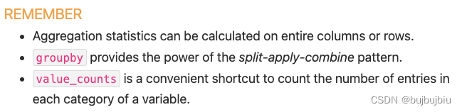
2.分组统计
乘客男性和女性的平均年龄分别是多少。使用titanic[["Sex", "Age"]]选中年龄和性别两列,对Sex列执行groupby创建分组,最后返回每个分组的年龄均值。对组计算统计值是一个split-apply-combine过程
- Split the data into groups
- Apply a function to each group independently
- Combine the results into a data structure
>>> titanic[['Sex','Age']].groupby('Sex').mean()
              Age
Sex
female  27.915709
male    30.726645
如果不选择指定的两列,对所有列计算性别分组后的均值,由于存在文本数据,传入参数numeric_only=True只计算数字。但是对Pclass计算均值无意义,通常需要指定某些列
>>> titanic.groupby('Sex').mean(numeric_only=True)
        PassengerId  Survived    Pclass  ...     SibSp     Parch       Fare
Sex                                      ...
female   431.028662  0.742038  2.159236  ...  0.694268  0.649682  44.479818
male     454.147314  0.188908  2.389948  ...  0.429809  0.235702  25.523893

[2 rows x 7 columns]
计算每种性别的平均年龄也可以先对整体数据分布然后选择Age列
>>> titanic.groupby('Sex')['Age'].mean()
Sex
female    27.915709
male      30.726645
Name: Age, dtype: float64

每个性别和舱位组合的平均票价是多少,groupby也可以对多列同时分组,传入列名的列表
>>> titanic.groupby(["Sex", "Pclass"])['Fare'].mean()
Sex     Pclass
female  1         106.125798
        2          21.970121
        3          16.118810
male    1          67.226127
        2          19.741782
        3          12.661633
Name: Fare, dtype: float64
3.按类别计算条目数
想要知道每类舱位的乘客数量使用value_counts()
>>> titanic['Pclass'].value_counts()
3    491
1    216
2    184
Name: Pclass, dtype: int64
value_counts()实际上是先分组后计数,等效于下面的操作
>>> titanic.groupby('Pclass')['Pclass'].count()
Pclass
1    216
2    184
3    491
Name: Pclass, dtype: int64
size和count都能和groupby配合使用,size包含空值,count去除了缺失值
(七)如何重新设计表格的布局
需要用到两个数据集titanic.csv和air_quality_long.csv
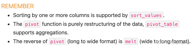
1.对表格行排序
根据乘客年龄对Titanic data进行排序sort_values()
>>> titanic.sort_values(by='Age').head()
     PassengerId  Survived  Pclass  ...     Fare Cabin  Embarked
803          804         1       3  ...   8.5167   NaN         C
755          756         1       2  ...  14.5000   NaN         S
644          645         1       3  ...  19.2583   NaN         C
469          470         1       3  ...  19.2583   NaN         C
78            79         1       2  ...  29.0000   NaN         S

[5 rows x 12 columns]
根据舱位和年龄降序排列
>>> titanic.sort_values(by=['Pclass','Age'],ascending=False).head()
     PassengerId  Survived  Pclass  ...    Fare Cabin  Embarked
851          852         0       3  ...  7.7750   NaN         S
116          117         0       3  ...  7.7500   NaN         Q
280          281         0       3  ...  7.7500   NaN         Q
483          484         1       3  ...  9.5875   NaN         S
326          327         0       3  ...  6.2375   NaN         S

[5 rows x 12 columns]
2.long to wide table
使用空气质量数据的一小部分,air_quality['parameter'] == 'no2'取no2的数据,按照location分组,只使用每个分组的前两条数据
>>> air_quality = pd.read_csv('/Users/bujibujibiu/Desktop/air_quality_long.csv', index_col='date.utc', parse_dates=True)
>>> no2 = air_quality[air_quality['parameter'] == 'no2']
>>> no2_subset = no2.sort_index().groupby(['location']).head(2)
>>> no2_subset
                                city country  ... value   unit
date.utc                                      ...
2019-04-09 01:00:00+00:00  Antwerpen      BE  ...  22.5  µg/m³
2019-04-09 01:00:00+00:00      Paris      FR  ...  24.4  µg/m³
2019-04-09 02:00:00+00:00     London      GB  ...  67.0  µg/m³
2019-04-09 02:00:00+00:00  Antwerpen      BE  ...  53.5  µg/m³
2019-04-09 02:00:00+00:00      Paris      FR  ...  27.4  µg/m³
2019-04-09 03:00:00+00:00     London      GB  ...  67.0  µg/m³

[6 rows x 6 columns]
并排显示这三个位置的value ,pivot()函数改变数据的形状:每个索引/列组合都需要一个值。
>>> no2_subset.pivot(columns='location', values='value')
location                   BETR801  FR04014  London Westminster
date.utc
2019-04-09 01:00:00+00:00     22.5     24.4                 NaN
2019-04-09 02:00:00+00:00     53.5     27.4                67.0
2019-04-09 03:00:00+00:00      NaN      NaN                67.0
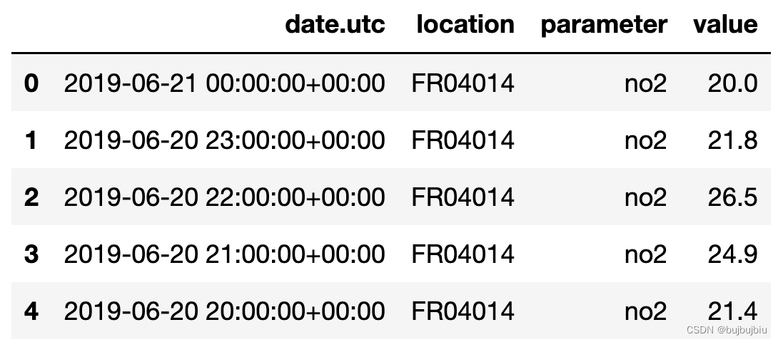
使用pivot()绘制每个位置的的value 图
>>> no2.head()
                            city country location parameter  value   unit
date.utc
2019-06-21 00:00:00+00:00  Paris      FR  FR04014       no2   20.0  µg/m³
2019-06-20 23:00:00+00:00  Paris      FR  FR04014       no2   21.8  µg/m³
2019-06-20 22:00:00+00:00  Paris      FR  FR04014       no2   26.5  µg/m³
2019-06-20 21:00:00+00:00  Paris      FR  FR04014       no2   24.9  µg/m³
2019-06-20 20:00:00+00:00  Paris      FR  FR04014       no2   21.4  µg/m³
>>> no2.pivot(columns='location',values='value').plot()

3.数据透视表
用表格形式显示每个地点的no2和pm2.5的均值,在pivot()中,数据被重新排列,但是在pivot_table()中可以传入aggfunc参数实现数据统计值的汇总
>>> air_quality.pivot_table(values='value', index='location', columns='parameter', aggfunc='mean')
parameter                 no2       pm25
location
BETR801             26.950920  23.169492
FR04014             29.374284        NaN
London Westminster  29.740050  13.443568
数据透视表pivot table是电子表格软件中众所周知的概念,如果需要每列或者每行的数据均值,设置margins=True
>>> air_quality.pivot_table(values='value', index='location', columns='parameter', aggfunc='mean', margins=True)
parameter                 no2       pm25        All
location
BETR801             26.950920  23.169492  24.982353
FR04014             29.374284        NaN  29.374284
London Westminster  29.740050  13.443568  21.491708
All                 29.430316  14.386849  24.222743
使用下面的分组也能实现相同的结果
>>> air_quality.groupby(["parameter", "location"]).mean()
                                  value
parameter location
no2       BETR801             26.950920
          FR04014             29.374284
          London Westminster  29.740050
pm25      BETR801             23.169492
          London Westminster  13.443568
4.wide to long table
使用前面的no2透视表,reset_index()重置索引
>>> no_pivoted = no2.pivot(columns='location', values='value').reset_index()
>>> no_pivoted.head()
location                  date.utc  BETR801  FR04014  London Westminster
0        2019-04-09 01:00:00+00:00     22.5     24.4                 NaN
1        2019-04-09 02:00:00+00:00     53.5     27.4                67.0
2        2019-04-09 03:00:00+00:00     54.5     34.2                67.0
3        2019-04-09 04:00:00+00:00     34.5     48.5                41.0
4        2019-04-09 05:00:00+00:00     46.5     59.5                41.0
想要收集所有的空气质量no2值在单一列,melt()函数将数据表从wide形式转化成long形式,
>>> no_2 = no_pivoted.melt(id_vars='date.utc')
>>> no_2.head()
                   date.utc location  value
0 2019-04-09 01:00:00+00:00  BETR801   22.5
1 2019-04-09 02:00:00+00:00  BETR801   53.5
2 2019-04-09 03:00:00+00:00  BETR801   54.5
3 2019-04-09 04:00:00+00:00  BETR801   34.5
4 2019-04-09 05:00:00+00:00  BETR801   46.5
传入到melt中的参数可以更详细
>>> no_2 = no_pivoted.melt(id_vars="date.utc", value_vars=["BETR801", "FR04014", "London Westminster"], value_name="NO_2", var_name="id_location")
>>> no_2.head()
                   date.utc id_location  NO_2
0 2019-04-09 01:00:00+00:00     BETR801  22.5
1 2019-04-09 02:00:00+00:00     BETR801  53.5
2 2019-04-09 03:00:00+00:00     BETR801  54.5
3 2019-04-09 04:00:00+00:00     BETR801  34.5
4 2019-04-09 05:00:00+00:00     BETR801  46.5
(八)如何从多个表格连接数据
使用两个数据集air_quality_no2_long.csv和air_quality_pm25_long.csv
>>> air_quality_no2 = pd.read_csv('/Users/bujibujibiu/Desktop/air_quality_no2_long.csv', parse_dates=True)
>>> air_quality_no2 = air_quality_no2[['date.utc', 'location', 'parameter', 'value']]
>>> air_quality_no2.head()
>>> air_quality_pm25 = pd.read_csv('/Users/bujibujibiu/Desktop/air_quality_pm25_long.csv', parse_dates=True)
>>> air_quality_pm25 = air_quality_pm25[['date.utc', 'location', 'parameter', 'value']]
>>> air_quality_pm25.head()

1.直接连接concat()

直接合并两个表成一个表使用concat(),concat()沿着某轴执行表的连接操作,按行或者按列,默认axis=0(行),因此结果是输入表格行的连接,查看表维度可知结果有3178=1110+2068行,按行连接因此是4列,基于日期进行排序也能看到两个表格确实合并了
>>> air_quality = pd.concat([air_quality_pm25, air_quality_no2], axis=0)
>>> air_quality = air_quality.sort_values('date.utc')
>>> air_quality.head()

>>> print('Shape of the ``air_quality_pm25`` table: ', air_quality_pm25.shape)
Shape of the ``air_quality_pm25`` table:  (1110, 4)
>>> print('Shape of the ``air_quality_no2`` table: ', air_quality_no2.shape)
Shape of the ``air_quality_no2`` table:  (2068, 4)
>>> print('Shape of the resulting ``air_quality`` table: ', air_quality.shape)
Shape of the resulting ``air_quality`` table:  (3178, 4)
在这个例子中,两个表格的parameter值完全不同,可以区分,但是情况不总是如此,concat函数也提供了key参数,添加额外的行索引,
>>> air_quality = pd.concat([air_quality_pm25, air_quality_no2], keys=["PM25", "NO2"])
>>> air_quality.head()

2.使用公共索引连接表格merge()
使用数据集air_quality_stations.csv
>>> stations_coord = pd.read_csv('/Users/bujibujibiu/Desktop/air_quality_stations.csv')
>>> stations_coord.head()
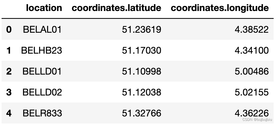
将stations_coord和air_quality按照location进行左连接,使用merge()函数,对于air_quality中的每行,从stations_coord表中找到对于location的行,how表示连接方式,和数据库类似,左连接表示只保留air_quality中的位置,如FR04014, BETR801,London Westminster,还支持其它连接方式,如右连接,全连接
>>> air_quality = pd.merge(air_quality, stations_coord, how='left', on='location')
>>> air_quality.head()

使用数据集air_quality_parameters.csv
>>> air_quality_parameters = pd.read_csv('/Users/bujibujibiu/Desktop/air_quality_parameters.csv')
>>> air_quality_parameters.head()

连接air_quality_parameters和air_quality,两个表格没有共同列,但是air_quality中的parameter和air_quality_parameters中的id两列有相同的变量,使用left_on和right_on可连接两表
>>> air_quality = pd.merge(air_quality, air_quality_parameters, how='left', left_on='parameter', right_on='id')
>>> air_quality.head()

(九)如何处理时间序列数据
使用数据集air_quality_no2_long
>>> air_quality = pd.read_csv('/Users/bujibujibiu/Desktop/air_quality_no2_long.csv')
>>> air_quality = air_quality.rename(columns={

    "date.utc": "datetime"})
>>> air_quality.head()

>>> air_quality.city.unique()
array(['Paris', 'Antwerpen', 'London'], dtype=object)
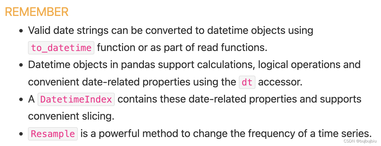
1.使用pandas datetime属性
首先先把datetime列转化成datetime对象,现在datetime列是字符类型,无法进行时间序列操作,通过to_datetime能将字符串转化为如pandas.Timestamp类型
>>> air_quality['datetime'] = pd.to_datetime(air_quality['datetime'])
>>> air_quality['datetime']
0      2019-06-21 00:00:00+00:00
1      2019-06-20 23:00:00+00:00
2      2019-06-20 22:00:00+00:00
3      2019-06-20 21:00:00+00:00
4      2019-06-20 20:00:00+00:00
                  ...
2063   2019-05-07 06:00:00+00:00
2064   2019-05-07 04:00:00+00:00
2065   2019-05-07 03:00:00+00:00
2066   2019-05-07 02:00:00+00:00
2067   2019-05-07 01:00:00+00:00
Name: datetime, Length: 2068, dtype: datetime64[ns, UTC]
使用pandas.Timestamp可以执行各种操作,如找到开始和结束时间以及时间跨度
>>> air_quality['datetime'].max() - air_quality['datetime'].min()
Timedelta('44 days 23:00:00')
增加新列只保留月份
air_quality['month'] = air_quality['datetime'].dt.month
air_quality.head()

每个location在一周的每天的平均no2浓度,对于每天使用weekday属性(monday=0,sunday=6),Timestamp的dt属性可以单独取年月日等
air_quality.groupby([air_quality['datetime'].dt.weekday, 'location'])['value'].mean()

计算每小时的no2平均值并绘图,先按hour分组取value列均值然后绘图
fig,axs = plt.subplots(figsize=(12,4))
air_quality.groupby(air_quality['datetime'].dt.hour)['value'].mean().plot(kind='bar',rot=0,ax=axs)

2.使用Datetime作为索引
前文提到可以用pivot()转换表格样式把每个地点no2值单独作为一列,通常把某列设置成索引可以使用set_index()
no_2 = air_quality.pivot(index='datetime', columns='location', values='value')
no_2.head()

使用DatetimeIndex可以执行很多函数,不在需要dt
>>> no_2.index.year, no_2.index.weekday
(Int64Index([2019, 2019, 2019, 2019, 2019, 2019, 2019, 2019, 2019, 2019,
             ...
             2019, 2019, 2019, 2019, 2019, 2019, 2019, 2019, 2019, 2019],
            dtype='int64', name='datetime', length=1033),
 Int64Index([1, 1, 1, 1, 1, 1, 1, 1, 1, 1,
             ...
             3, 3, 3, 3, 3, 3, 3, 3, 3, 4],
            dtype='int64', name='datetime', length=1033))
选取时序子集也比较方便,如绘制某一区间不同地点的no2值
no_2["2019-05-20":"2019-05-21"].plot()

3.将时间序列重新采样到另一个频率
按月分组后保留最大值resample()
monthly_max = no_2.resample('M').max()
monthly_max

绘制每个地点每天的no2均值
no_2.resample('D').mean().plot(style='-o',figsize=(10,5))

(十)如何处理文本数据
使用数据集titanic.csv
乘客姓名换成小写,选择str后再执行操作,和时间序列的dt功能相同
>>> titanic['Name'].str.lower()
0                                braund, mr. owen harris
1      cumings, mrs. john bradley (florence briggs th...
2                                 heikkinen, miss. laina
3           futrelle, mrs. jacques heath (lily may peel)
4                               allen, mr. william henry
                             ...
886                                montvila, rev. juozas
887                         graham, miss. margaret edith
888             johnston, miss. catherine helen "carrie"
889                                behr, mr. karl howell
890                                  dooley, mr. patrick
Name: Name, Length: 891, dtype: object
创建Surname列包含每个乘客的名,先使用Series.str.split()将Name列变成列表,然后取第一个元素即名get(),所有对字符串进行操作都是基于str
>>> titanic['Name'].str.split(',')
0                             [Braund,  Mr. Owen Harris]
1      [Cumings,  Mrs. John Bradley (Florence Briggs ...
2                              [Heikkinen,  Miss. Laina]
3        [Futrelle,  Mrs. Jacques Heath (Lily May Peel)]
4                            [Allen,  Mr. William Henry]
                             ...
886                             [Montvila,  Rev. Juozas]
887                      [Graham,  Miss. Margaret Edith]
888          [Johnston,  Miss. Catherine Helen "Carrie"]
889                             [Behr,  Mr. Karl Howell]
890                               [Dooley,  Mr. Patrick]
Name: Name, Length: 891, dtype: object
>>> titanic['Surname'] = titanic['Name'].str.split(',').str.get(0)
>>> titanic['Surname']
0         Braund
1        Cumings
2      Heikkinen
3       Futrelle
4          Allen
         ...
886     Montvila
887       Graham
888     Johnston
889         Behr
890       Dooley
Name: Surname, Length: 891, dtype: object
提取有关泰坦尼克号上伯爵夫人的乘客数据,使用contains()筛选名字
>>> titanic['Name'].str.contains('Countess')
0      False
1      False
2      False
3      False
4      False
       ...
886    False
887    False
888    False
889    False
890    False
Name: Name, Length: 891, dtype: bool
>>> titanic[titanic['Name'].str.contains('Countess')]
     PassengerId  Survived  Pclass  ... Cabin Embarked  Surname
759          760         1       1  ...   B77        S   Rothes

[1 rows x 13 columns]
乘客里谁的名字最长?titanic['Name'].str.len()显示名字长度,idxmax()找到最大值的索引,loc找到最长名字
>>> titanic['Name'].str.len()
0      23
1      51
2      22
3      44
4      24
       ..
886    21
887    28
888    40
889    21
890    19
Name: Name, Length: 891, dtype: int64
>>> titanic['Name'].str.len().idxmax()
307
>>> titanic.loc[titanic['Name'].str.len().idxmax(), 'Name']
'Penasco y Castellana, Mrs. Victor de Satode (Maria Josefa Perez de Soto y Vallejo)'
新增Sex_short(),用M代替male,F代替female,替代操作使用replace()
>>> titanic['Sex_short'] = titanic['Sex'].replace({

    'male':'M','female':'F'})
>>> titanic['Sex_short']
0      M
1      F
2      F
3      F
4      M
      ..
886    M
887    F
888    F
889    M
890    M
Name: Sex_short, Length: 891, dtype: object
分开操作和下面代码功能相同,但是顺序不能改变,因为female包含male
titanic["Sex_short"] = titanic["Sex"].str.replace("female", "F")
titanic["Sex_short"] = titanic["Sex_short"].str.replace("male", "M")
总结