基于 LSTM 进行多类文本分类（ TensorFlow 2.0）

NLP 的许多创新是如何将上下文添加到词向量中。一种常见的方法是使用循环神经网络。以下是循环神经网络的概念：

他们利用顺序信息。
他们可以捕捉到到目前为止已经计算过的内容，即：我最后说的内容会影响我接下来要说的内容。
RNNs 是文本和语音分析的理想选择。
最常用的 RNNs 是 LSTM。

来源：https://colah.github.io/posts/2015-08-Understanding-LSTMs/

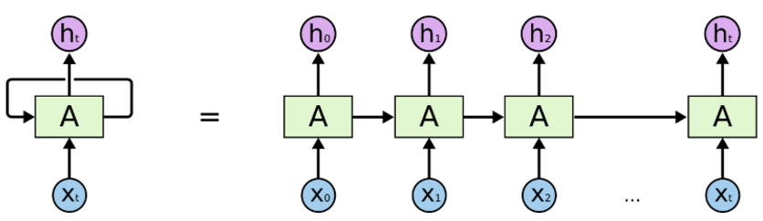
以上是循环神经网络的架构：

“A”是一层前馈神经网络。
如果我们只看右边，它确实会循环通过每个序列的元素。
如果我们打开左边，它看起来就像右边。

来源：https://colah.github.io/posts/2015-08-Understanding-LSTMs

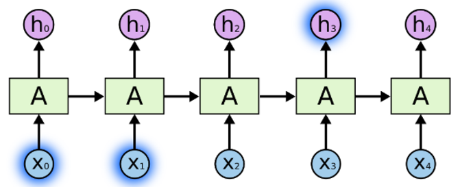
假设我们正在解决新闻文章数据集的文档分类问题：

我们输入每个单词，单词以某种方式相互关联。
当我们看到那篇文章中的所有单词时，我们会在文章末尾做出预测。
RNNs 通过传递来自最后输出的输入，能够保留信息，并能够在最后利用所有信息进行预测。

https://colah.github.io/posts/2015-08-Understanding-LSTMs

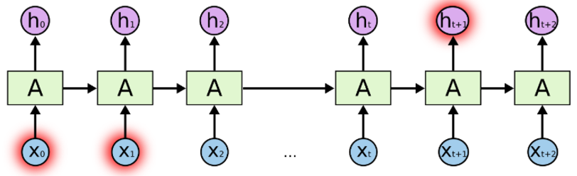
这适用于短句，当我们处理长文章时，会出现长期依赖问题。

因此，我们一般不使用 vanilla RNN，而是使用 Long Short Term Memory。LSTM 是一种可以解决这种长期依赖问题的 RNN。

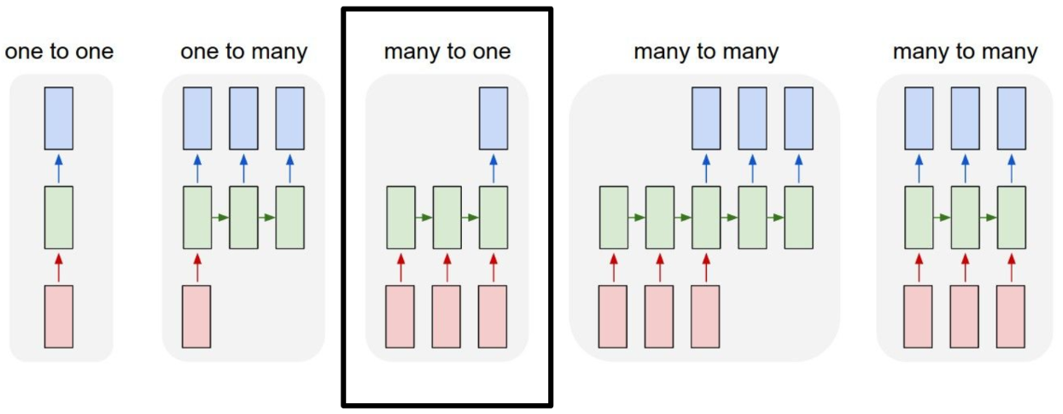
在我们的新闻文章文档分类示例中，我们有这种多对一的关系。输入是单词序列，输出是单个类或标签。

现在我们将使用 TensorFlow 2.0 和 Keras，基于 LSTM 解决 BBC 新闻文档分类问题。

数据链接：https://raw.githubusercontent.com/susanli2016/PyCon-Canada-2019-NLP-Tutorial/master/bbc-text.csv

首先，我们导入相关库并确保我们的 TensorFlow 是正确的版本。

import csv
import tensorflow as tf
import numpy as np
from tensorflow.keras.preprocessing.text import Tokenizer
from tensorflow.keras.preprocessing.sequence import pad_sequences
from nltk.corpus import stopwords
STOPWORDS = set(stopwords.words('english'))


print(tf.__version__)

2.0.0

像这样将超参数放在顶部，以便更容易更改和编辑。
当我们用到时，再解释每个超参数是如何工作的。

vocab_size = 5000
embedding_dim = 64
max_length = 200
trunc_type = 'post'
padding_type = 'post'
oov_tok = '<OOV>'
training_portion = .8

hyperparamenter.py

定义两个包含文章和标签的列表。，与此同时，我们过滤掉了停用词。

articles = []
labels = []


with open("bbc-text.csv", 'r') as csvfile:
    reader = csv.reader(csvfile, delimiter=',')
    next(reader)
    for row in reader:
        labels.append(row[0])
        article = row[1]
        for word in STOPWORDS:
            token = ' ' + word + ' '
            article = article.replace(token, ' ')
            article = article.replace(' ', ' ')
        articles.append(article)
print(len(labels))
print(len(articles))

articles_labels.py

2225

数据中有 2225 篇新闻文章，我们将它们分为训练集和验证集，根据我们之前设置的参数，80% 用于训练，20% 用于验证。

train_size = int(len(articles) * training_portion)


train_articles = articles[0: train_size]
train_labels = labels[0: train_size]


validation_articles = articles[train_size:]
validation_labels = labels[train_size:]


print(train_size)
print(len(train_articles))
print(len(train_labels))
print(len(validation_articles))
print(len(validation_labels))

train_valid.py

1780

445

Tokenizer 为我们完成了所有繁重的工作。在我们对其进行标记的文章中，它将使用 5,000 个最常用的单词。oov_token 是在遇到看不见的单词时放入一个特殊值。这意味着我们希望用于不在 word_index 中的单词。fit_on_text 将遍历所有文本并创建如下字典：

tokenizer = Tokenizer(num_words = vocab_size, oov_token=oov_tok)
tokenizer.fit_on_texts(train_articles)
word_index = tokenizer.word_index
dict(list(word_index.items())[0:10])

tokenize.py

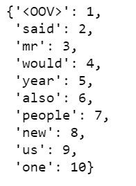
我们可以看到“”是我们语料库中最常见的标记，其次是“said”，然后是“mr”等等。

标记化之后，下一步是将这些标记转换为序列列表。以下是已转为序列的训练数据中的第 11 篇文章。

train_sequences = tokenizer.texts_to_sequences(train_articles)
print(train_sequences[10])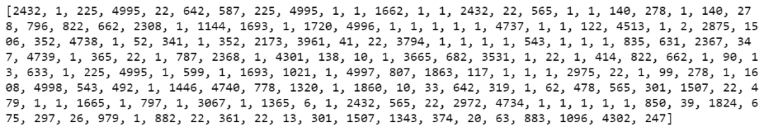

当我们为 NLP 训练神经网络时，我们需要数据长度大小相同，这就是我们使用填充的原因。如果你查一下，我们的 max_length 是 200，所以我们使用 pad_sequences 使我们所有文章的长度都相同，即 200。结果，你会看到第 1 篇文章的长度是 426，它变成了 200，第 2 篇文章长度为 192，变为 200，依此类推。

train_padded = pad_sequences(train_sequences, maxlen=max_length, padding=padding_type, truncating=trunc_type)
print(len(train_sequences[0]))
print(len(train_padded[0]))


print(len(train_sequences[1]))
print(len(train_padded[1]))


print(len(train_sequences[10]))
print(len(train_padded[10]))

425

200

192

200

186

200

此外，还有padding_type和truncating_type，都有所有帖子，例如，对于第11篇文章，长度为186，我们填充了200个，我们在末端填充了14个零。

print(train_padded[10])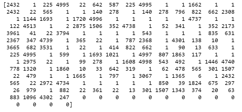

对于第一篇文章，它的长度为426，我们截断为200。

然后，我们为验证集合做同样的事情。

validation_sequences = tokenizer.texts_to_sequences(validation_articles)
validation_padded = pad_sequences(validation_sequences, maxlen=max_length, padding=padding_type, truncating=trunc_type)


print(len(validation_sequences))
print(validation_padded.shape)

445

（445， 200）

现在，我们将查看标签。因为我们的标签是文本，所以我们将在训练时将其贴上标签，预计标签将为Numpy矩阵。因此，我们将标签列表变成像这样的Numpy矩阵格式：

label_tokenizer = Tokenizer()
label_tokenizer.fit_on_texts(labels)


training_label_seq = np.array(label_tokenizer.texts_to_sequences(train_labels))
validation_label_seq = np.array(label_tokenizer.texts_to_sequences(validation_labels))
print(training_label_seq[0])
print(training_label_seq[1])
print(training_label_seq[2])
print(training_label_seq.shape)


print(validation_label_seq[0])
print(validation_label_seq[1])
print(validation_label_seq[2])
print(validation_label_seq.shape)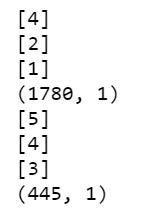

在训练深度神经网络之前，我们可以抽查原始文章和填充后的文章。运行以下代码，我们查看了第11篇文章，我们可以看到有些单词变成“”，因为它们没有进入前5,000名。

reverse_word_index = dict([(value, key) for (key, value) in word_index.items()])


def decode_article(text):
    return ' '.join([reverse_word_index.get(i, '?') for i in text])
print(decode_article(train_padded[10]))
print('---')
print(train_articles[10])

现在是训练LSTM的时候了。

我们构建一个tf.keras.Sequential模型，并从 embeddings 开始。一个 embeddings 将每个单词存储为一个矢量。当调用时，它将单词索引序列转换为向量序列。训练后，具有相似含义的单词通常具有相似的向量。
Bidirectional wrapper 与LSTM层一起使用，这可以通过LSTM层向前和向后传播输入，然后将输出串联。这有助于LSTM学习长期依赖性。
我们使用 relu 代替 tahn。
我们添加一个具有6个单元和 SoftMax 函数。当我们有多个输出时，SoftMax 将输出层转换为概率分布。

model = tf.keras.Sequential([
    # Add an Embedding layer expecting input vocab of size 5000, and output embedding dimension of size 64 we set at the top
    tf.keras.layers.Embedding(vocab_size, embedding_dim),
    tf.keras.layers.Bidirectional(tf.keras.layers.LSTM(embedding_dim)),
#    tf.keras.layers.Bidirectional(tf.keras.layers.LSTM(32)),
    # use ReLU in place of tanh function since they are very good alternatives of each other.
    tf.keras.layers.Dense(embedding_dim, activation='relu'),
    # Add a Dense layer with 6 units and softmax activation.
    # When we have multiple outputs, softmax convert outputs layers into a probability distribution.
    tf.keras.layers.Dense(6, activation='softmax')
])
model.summary()

在我们的模型 summary 中，我们有 embeddings，Bidirectional LSTM，然后是两个 dense 层。双向的输出为128，因为它使我们在LSTM中输入的输出增加了一倍。我们也可以堆叠LSTM层，但我发现结果更糟。

print(set(labels))

我们总共有5个标签，但是由于我们没有使用 one-hot 编码标签，因此我们必须使用 sparse_categorical_crossentropy 作为损失函数，因此似乎也认为0也是一个可能的标签。因此，最后一个密集层需要标签0、1、2、3、4、5的输出，而不是整数，尽管从未使用过0。

如果您希望最后一个密集的层是5，则需要从训练集和验证集的标签中减去1。（此处保留）

我决定训练10个epoch。

model.compile(loss='sparse_categorical_crossentropy', optimizer='adam', metrics=['accuracy'])
num_epochs = 10
history = model.fit(train_padded, training_label_seq, epochs=num_epochs, validation_data=(validation_padded, validation_label_seq), verbose=2)

def plot_graphs(history, string):
  plt.plot(history.history[string])
  plt.plot(history.history['val_'+string])
  plt.xlabel("Epochs")
  plt.ylabel(string)
  plt.legend([string, 'val_'+string])
  plt.show()
  
plot_graphs(history, "accuracy")
plot_graphs(history, "loss")

我们可能只需要3或4个epoch。（在训练结束时，我们可以看到有点过于拟合）

· END ·

HAPPY LIFE

基于 LSTM 进行多类文本分类（ TensorFlow 2.0）

猜你喜欢